Picking random regression lines from the distribution of OLS regressions

Question

I regressed a series of data with OLS, and I calculated the standard error (SE) of the slope and of the intercept. Moreover, I calculated the confidence bands for the regression following the equations in the answer to this question. Now I am wondering how I can generate a set of random regression lines within this distribution of regression lines that is illustrated by the 95% confidence interval.

In order to illustrate what I mean, here is a short summary of my problem. I have a series of data (dataset A; blue points in below figure) that deviate from a linear trend defined by another dataset (dataset B; red points in below figure). Using some constraints from chemistry, I can correct A by projecting each point onto the linear trend defined by B (red regression line in below figure). In order to consider the uncertainty in the regression of dataset B in the corrected values for dataset A, I was thinking of picking lines at random from the distribution of regressions of dataset B, and projecting A onto each of these lines. I just do not know how to pick lines that are representative of the distribution of regressions.

Below is now a zoom into the same plot as above. Now, the black lines show 100 regression lines picked at random. These lines were generated by choosing random values for the slope and intercept from normal distributions with mean and standard errors obtained from the regression.

Here is the same with 1000 lines

There seem to be more than 5% of the lines that fall out of the 95% confidence bands, and the method of picking a random slope and a random intercept value does not work. This makes sense, considering that slope and intercept are not independent. Is there a simple way to generate regressions that are representative of the true distribution of regression lines around the "best fit"?

Thanks and please let me know if any of this is unclear

Answer 1

In a linear regression model, the joint sampling distribution of the model parameters is described in this post and this one. Specifically, $$ \hat{\beta}\;|\;X\sim \mathrm{N}\left(\beta, \sigma^{2}(X^TX)^{-1}\right) $$ where $X$ is the design matrix. In a simple linear regression with only one predictor and an intercept, the design matrix has dimensions $N\times 2$ (i.e. it has two columns and $N$ rows) where $N$ is the sample size. You could then sample from a bivariate normal distribution to generate regression lines. Another possibility would be to bootstrap.

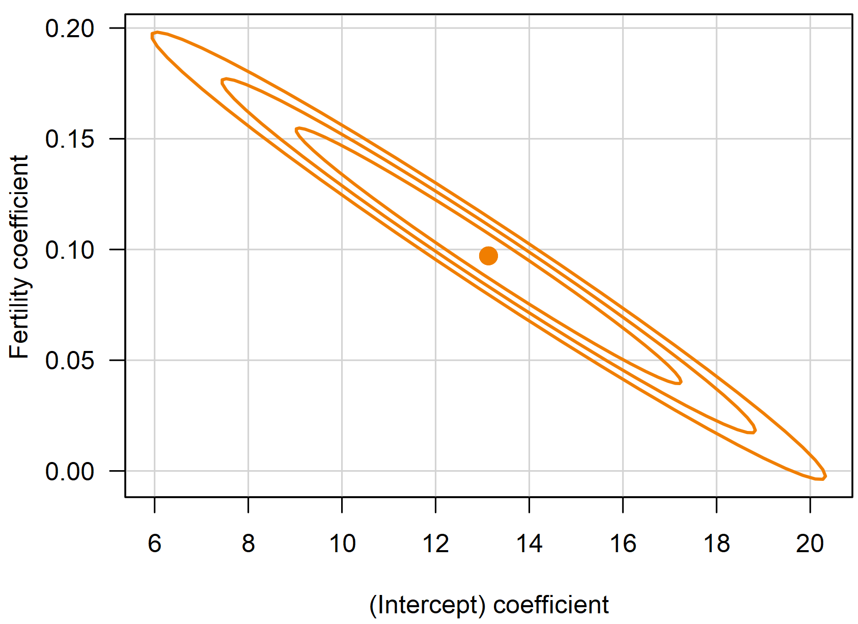
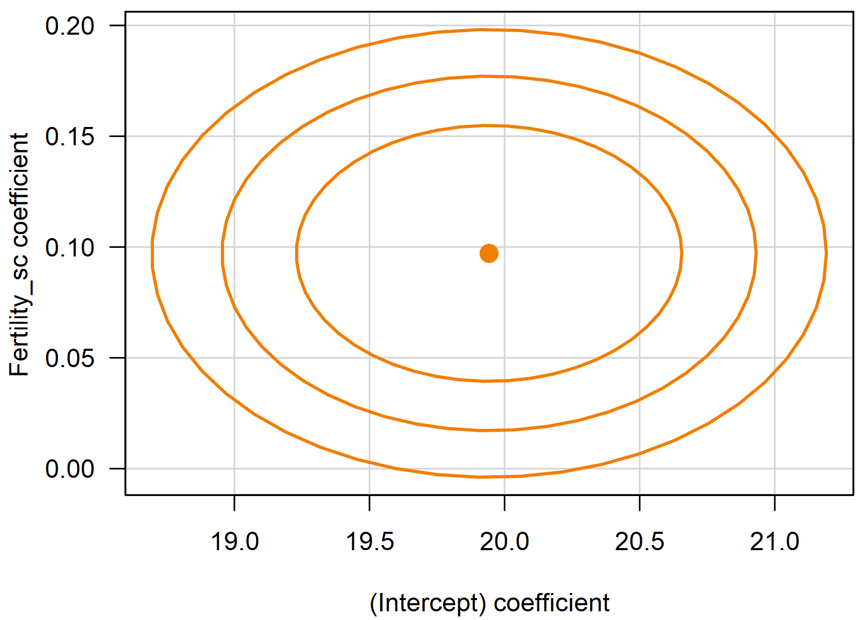
If the predictor variable was centered on its sample mean before the regression, then the covariance between the intercept and the slope is $0$ (for more information, look here). More general: If the sample mean of the predictor variable $x$ is not $0$ ($\bar{x}\neq 0$), the intercept and the slope are correlated. If the predictor variable was not centered, the intercept and the slope are not independent. The following graphic depicts the 80%, 95% and 99% confidence ellipse for the slope and the intercept in the case that the predictor variable was not centered:

If the predictor were centered, the corresponding confidence ellipses look different:

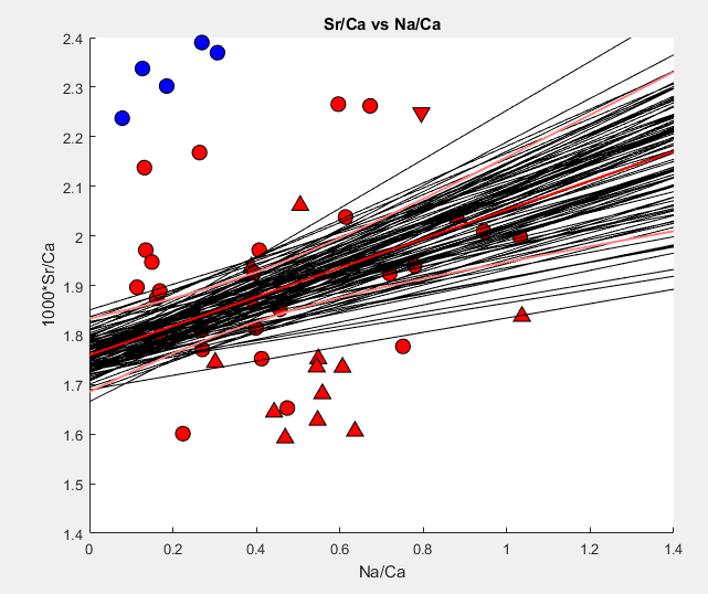
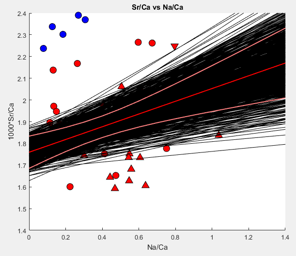
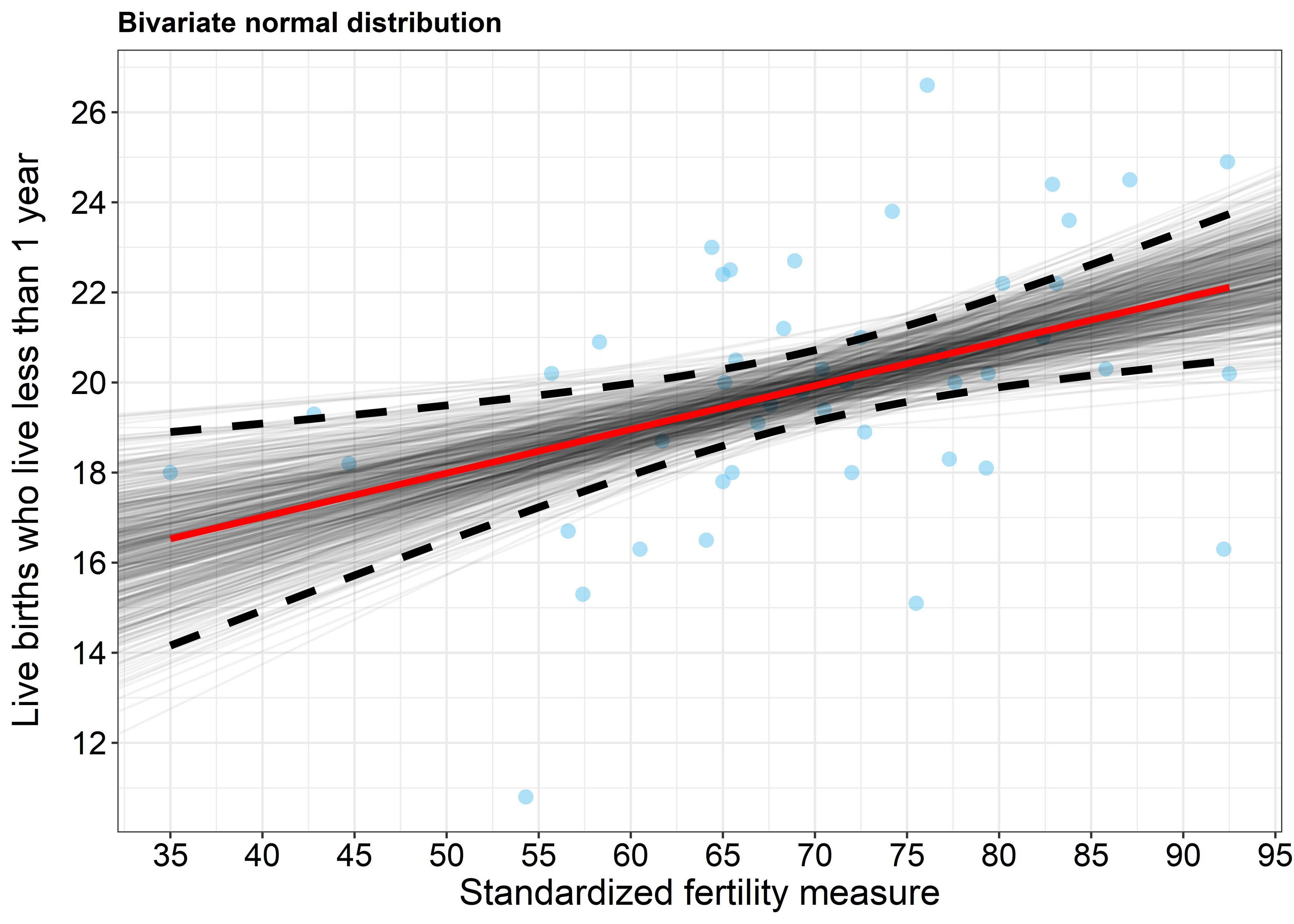
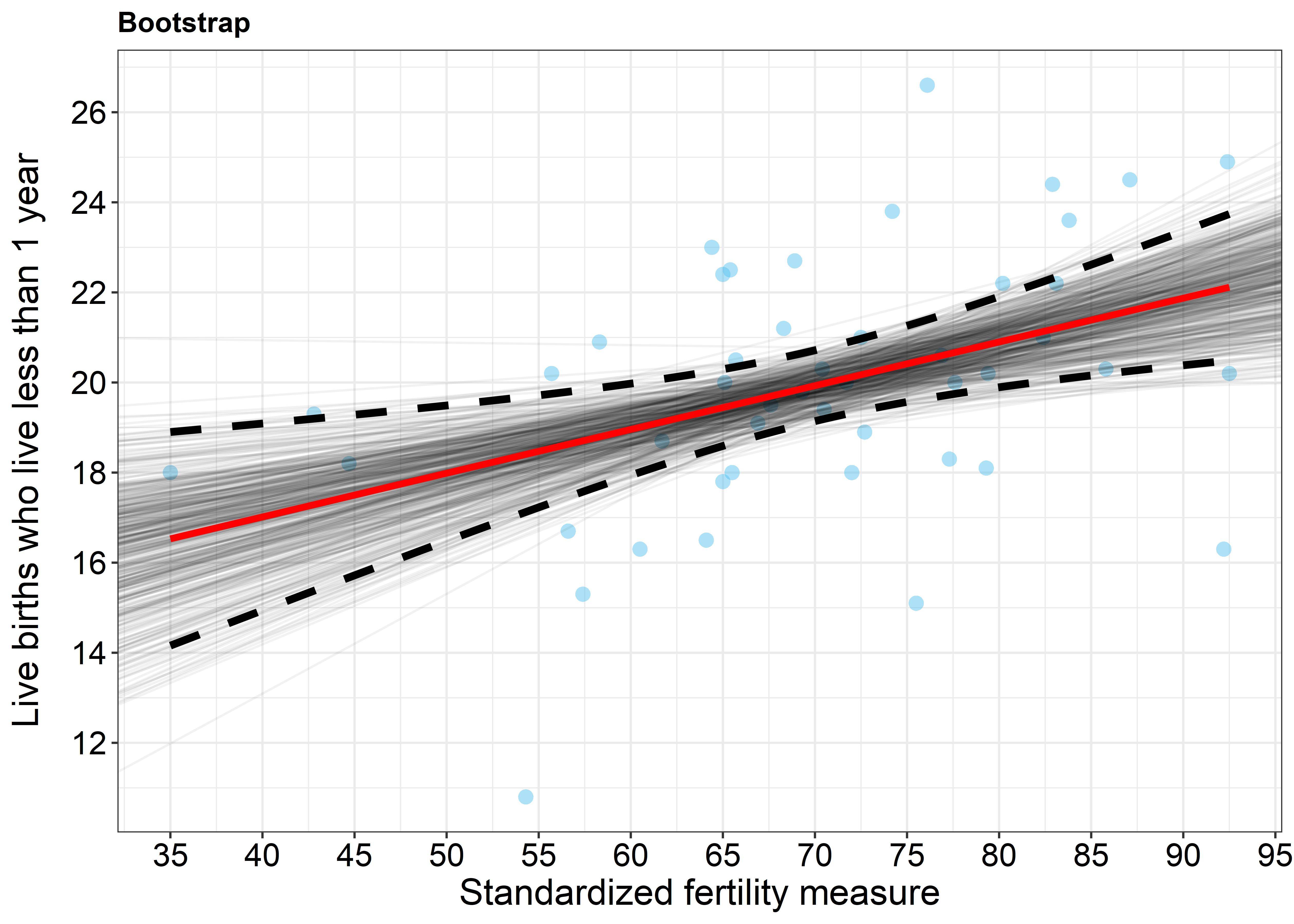
Here are two graphics, the first was generated by sampling 500 times from the bivariate normal distribution and the second one was generated by 500 nonparametric bootstrap replicates. The red line denotes the ols fit and the dashed black lines denote the 95% confidence intervals. The individual resampled regression lines are drawn in a translucent black so that the color is darker in regions were they overlap. You can see clearly that the majority of the resampled regression lines lie within the 95% confidence band, as we would expect.

Here is the R code I used:

library(MASS)
library(scales)
library(ggplot2)
library(reshape2)

mod <- lm(Infant.Mortality~Fertility, data = swiss)

Sigma <- vcov(mod) # The covariance matrix of the estimates
mu <- coef(mod) # The estimates

set.seed(142857)

n_sim <- 500      # Number of replicates

x <- mvrnorm(n = n_sim, mu = mu, Sigma = Sigma) # Sample from the bivariate normal distribution

rbind(x, c(mu))

plot_frame <- data.frame(
  int = x[, 1]
  , slope = x[, 2]
)

pred_frame <- data.frame(
  Fertility = seq(min(swiss$Fertility), max(swiss$Fertility), length.out = 1000)
)

pred_frame$lwr <- predict(mod, newdata = pred_frame, interval = "confidence")[, 2]
pred_frame$upr <- predict(mod, newdata = pred_frame, interval = "confidence")[, 3]


theme_set(theme_bw())
p <- ggplot(data = swiss, aes(x = Fertility, y = Infant.Mortality)) +
  geom_point(size = 3, colour = "#5CC3F0", alpha = 0.5, pch = 16) +
  geom_abline(data = plot_frame, aes(intercept = int, slope = slope), col = "black", alpha = 0.05) +
  geom_line(data = pred_frame, aes(x = Fertility, y = lwr), linetype = 2, size = 1.7) +
  geom_line(data = pred_frame, aes(x = Fertility, y = upr), linetype = 2, size = 1.7) +
  stat_smooth(method = "lm", se = FALSE, col = "red", size = 1.5, fullrange = TRUE) +
  xlab("Standardized fertility measure") +
  ylab("Live births who live less than 1 year") +
  ggtitle("Bivariate normal distribution") +
  scale_x_continuous(breaks = scales::pretty_breaks(n = 10)) +
  scale_y_continuous(breaks = scales::pretty_breaks(n = 10)) +
  theme(
    axis.title.y=element_text(colour = "black", size = 17, hjust = 0.5, margin=margin(0,12,0,0)),
    axis.title.x=element_text(colour = "black", size = 17),
    axis.text.x=element_text(colour = "black", size=15),
    axis.text.y=element_text(colour = "black", size=15),
    legend.position="right",
    legend.text=element_text(size=12.5),
    legend.key=element_blank(),
    plot.title = element_text(face = "bold"),
    strip.text.x=element_text(size=15)
  )

#===============================================================
# Bootstrap
#===============================================================

set.seed(142857)

n_boot <- 500 # Number of bootstrap replicates

boot_res <- matrix(NA, ncol = 2, nrow = n_boot) # Matrix to store the bootstrap coefficients

# Start the bootstrap

for (i in seq_len(n_boot)) {
  boot_res[i, ] <- coef(lm(Infant.Mortality~Fertility, data = swiss[sample(seq_len(dim(swiss)[1]), replace = TRUE), ]))
}

boot_res <- data.frame(boot_res)
names(boot_res) <- c("int", "slope")

theme_set(theme_bw())
p <- ggplot(data = swiss, aes(x = Fertility, y = Infant.Mortality)) +
  geom_point(size = 3, colour = "#5CC3F0", alpha = 0.5, pch = 16) +
  geom_abline(data = boot_res, aes(intercept = int, slope = slope), col = "black", alpha = 0.05) +
  geom_line(data = pred_frame, aes(x = Fertility, y = lwr), linetype = 2, size = 1.7) +
  geom_line(data = pred_frame, aes(x = Fertility, y = upr), linetype = 2, size = 1.7) +
  stat_smooth(method = "lm", se = FALSE, col = "red", size = 1.5, fullrange = TRUE) +
  xlab("Standardized fertility measure") +
  ylab("Live births who live less than 1 year") +
  ggtitle("Bootstrap") +
  scale_x_continuous(breaks = scales::pretty_breaks(n = 10)) +
  scale_y_continuous(breaks = scales::pretty_breaks(n = 10)) +
  theme(
    axis.title.y=element_text(colour = "black", size = 17, hjust = 0.5, margin=margin(0,12,0,0)),
    axis.title.x=element_text(colour = "black", size = 17),
    axis.text.x=element_text(colour = "black", size=15),
    axis.text.y=element_text(colour = "black", size=15),
    legend.position="right",
    legend.text=element_text(size=12.5),
    legend.key=element_blank(),
    plot.title = element_text(face = "bold"),
    strip.text.x=element_text(size=15)
  )