HELP: LM shows no relationship, but LMM does

Question

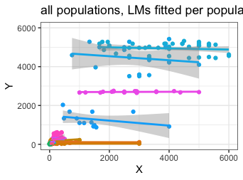
My research question is assessing if a variable (let’s call it ‘x') can predict another variable (let’s call it ‘y’). The two variables x and y are in the same units, but they just come from different sources of information. I have data on x and y for some 30 different populations in which values of x and y vary by as much as two orders of magnitude (simply because the populations are different; the data are believed to be as accurate as possible). For each population, values of x are generally close to y, suggesting that x can predict y. But, for each population, values of x show some variability, and values of y are often near-constant. X values show variability because they are individual-level observations and y values show little or no-variability because they are population averages. Unfortunately, for this research, it is impossible to obtain individual-level bservations of y, so I have no choice but to compare the two sets of variables.

In trying to address my research question, I have been using regression methods. This is what I have found so far:

1. When I do a simple linear regression for each population (separately) of y ~ x , I get that R2 is often near-zero, because y varies little. According to this post $R^2$ of linear regression with no variation in the response variable, this situation is one in which R2 is undefined. Note that this would still be the case even if x values did perfect predictions of y. See one example of my preliminary LM results for one such population below.

Call: lm(formula = y_pop1 ~ x_pop1, data = df_pop1)

Residuals:
   Min     1Q Median     3Q    Max 
-958.9 -674.2  -68.8  550.9 1091.7 

Coefficients:
             Estimate Std. Error t value Pr(>|t|)    
(Intercept) 4745.9153   488.7394   9.711 1.34e-07 ***
x.              -0.1039     0.1615  -0.643     0.53    
---
Signif. codes:  0 ‘***’ 0.001 ‘**’ 0.01 ‘*’ 0.05 ‘.’ 0.1 ‘ ’ 1

Residual standard error: 703.7 on 14 degrees of freedom
Multiple R-squared:  0.02872,   Adjusted R-squared:  -0.04066 
F-statistic: 0.4139 on 1 and 14 DF,  p-value: 0.5304

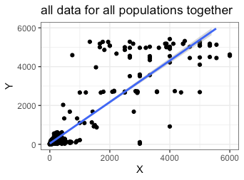
2. When I do a simple linear regression of y ~ x for all populations together, without accounting for each population (i.e., as a random effect), I get that R2 is high (~ 0.77). In this case, the relationship is due to the large difference in x and y values across all populations and the (somewhat) close agreement of x and y values within populations; these produce a (near) linear relationship, with increasing y values being followed by increasing x values. See preliminary LM results below. I cannot analyze my data this way, because I have different populations and need to account for differences among them. Such an analysis, I understand, would be subject to Simpson's Paradox (https://en.wikipedia.org/wiki/Simpson%27s_paradox).

Call:
lm(formula = y ~ x, data = df)

Residuals:
    Min      1Q  Median      3Q     Max 
-6110.1  -126.4  -105.3   -63.5  4061.0 

Coefficients:
             Estimate Std. Error t value Pr(>|t|)    
(Intercept) 118.43118   26.21227   4.518 7.18e-06 ***
x.               0.82621    0.01565  52.780  < 2e-16 ***
---
Signif. codes:  0 ‘***’ 0.001 ‘**’ 0.01 ‘*’ 0.05 ‘.’ 0.1 ‘ ’ 1

Residual standard error: 685.5 on 800 degrees of freedom
Multiple R-squared:  0.7769,    Adjusted R-squared:  0.7766 
F-statistic:  2786 on 1 and 800 DF,  p-value: < 2.2e-16

3. I have thus been trying to analyze my data using linear mixed models (LMM), where x predicts y and each population is a random effect. I am far from a statistician (or someone with strong understanding of statistics), but my understanding is that a LMM such as this one would assess if y can be predicted by x, while accounting for differences among populations. In other words, I believe this is the “right” approach for my analysis. Some preliminary LMM results are below, indicating that x does indeed predict y, though there is a tendency to under-estimate. Variable values for this LMM have been standardized (but the results are same when they are not standardized).

Linear mixed model fit by maximum likelihood  ['lmerMod']
Formula: y ~ x + (x - 1 | population)
   Data: datall

     AIC      BIC   logLik deviance df.resid 
   998.3   1017.1   -495.2    990.3      798 

Scaled residuals: 
    Min      1Q  Median      3Q     Max 
-8.2535 -0.1715 -0.0452  0.0185  5.5351 

Random effects:
 Groups   Name   Variance Std.Dev.
 Population   x      0.1453   0.3812  
 Residual              0.1906   0.4366  
Number of obs: 802, groups:  f.name, 33

Fixed effects:
             Estimate Std. Error t value
(Intercept)   0.20933    0.03785    5.53
x.                 1.39751    0.11417   12.24

Correlation of Fixed Effects:
            (Intr)
x.         0.651 

           R2m         R2c
      0.8532974    0.9167095

My question is whether the LMM above is producing misleading results given my points in 1 and 2. I would like to confirm that the LMM is indeed able to find relationships between x and y when considering and accounting for data for all populations together, even though LMs for each population separately cannot. IF there is a problem with such an analytical approach, I would be very interested in hearing alternative approaches to analyzing this data. I have not identified any so far.

Many thanks!