What to do when assumptions of both ANOVA and Kruskal-Wallis are violated?

Question

I am trying to analyse whether three groups (samples sizes 27, 26 and 23) differ in their responses to 20 questionnaire items, each measured using a 5-point likert scale. The items are all investigating different things, so it is not appropriate/of interest to condense them into likert scales for broader constructs.

I am well aware of the controversy surrounding the use of ANOVA for likert data. However, I have been advised that this could be justified, and I know of papers that suggest ANOVA is relatively robust in most situations. However, my data is also non-normal and contains multiple extreme outliers. As these outliers represent real likert responses, I believe that they have value and should not be excluded. Overall, I feel like there are a lot of arguments against using one-way ANOVAs to analyse the data at this point.

I have therefore also endeavoured to analyse the data using the Kruskal-Wallis test, which at first seemed to be more appropriate. However, the data violated the assumption that distributions across groups should be similar and consequently analysis can only tell me about the distributions of likert responses, rather than median responses which would make more interpretable sense (I think?). Following a guide to conducting and reporting the analysis, I arrived at findings like this: 'Likert ratings increased from Group 1 (mean rank = 33.78), to Group 2 (mean rank = 38.41), to Group 3 (mean rank = 42.77), but the differences were not statistically significant, χ2(2) = 2.218, p = .330.' Talking about 'mean rank' seems to be irrelevant to my discussion of whether, and in what ways, groups differed in their likert responses.

My supervisor is suggesting that I stick to one-way ANOVA, but I do not see how the results of this can be justified for this data. At the same time, Kruskel-Wallis does not seem suitable for my questions of interest.

I would greatly appreciate any advise on how I can best analyse my data at this point!

Answer 1

One of the difficulties of departing from the original measurement scale to find a suitable test is figuring out how to understand results on an unfamiliar, possibly unintuitive, measurement scale. If you get a suitably small P-value, then you can assert that there are significant differences among groups, but it can be difficult to assess whether these differences are large enough (on some scale) to be of practical interest.

Your sample sizes 27, 26, and 23 are modest, but it is worthwhile, as suggested by @jbowman, to investigate whether the Welch ANOVA (which does not assume equal variances) finds significant differences, and if so, what that means.

Simulated data. Below I generate fake data for three groups, in which subjects have somewhat different probabilities of choosing the various Likert values on a particular question. Specifically, responses 1 through 5 have proportions as follows--increasingly likely to choose higher values as we go from Group 1, to 2, to 3. (We could turn the 'proportions' into probabilities by dividing by 14, but it is not necessary to do so.)

p1 = c(1,3,5,3,2)
p2 = c(1,2,3,5,3)
p3 = c(1,1,2,5,5)

Then the Likert scores are generated in R as shown:

set.seed(1234)  # for reproducibility
x1 = sample(1:5, 27, rep=T, prob=p1)
x2 = sample(1:5, 26, rep=T, prob=p2)
x3 = sample(1:5, 23, rep=T, prob=p3)
x = c(x1,x2,x3)
g = as.factor(c(rep(1,27),rep(2,26),rep(3,23)))

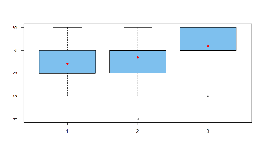
For an overview of these data, here are boxplots of the groups with red dots showing group means.

boxplot(x ~ g, col="skyblue2")
points(1:3, c(mean(x1), mean(x2), mean(x3)), 
  pch=19, col="red")

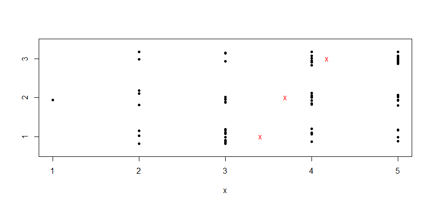
A stripchart shows the individual Likert scores. (Points have been 'jittered', randomly displaced vertically, to avoid plotting them directly on top of each other.)

stripchart(x ~ g, pch=20, meth="jit", jit=.2)
points(c(mean(x1), mean(x2), mean(x3)), 1:3, col="red", pch="x")

Group sample means differ and group sample variances also differ somewhat.

mean(x1); mean(x2); mean(x3)
[1] 3.407407
[1] 3.692308
[1] 4.173913
var(x1); var(x2); var(x3)
[1] 0.7891738
[1] 1.181538
[1] 0.9683794

So, it seems that I have simulated 'Likert' data with some differences in means among the groups. The question now is whether differences are large enough to rise significantly above the random noise.

Welch ANOVA. The Welch ANOVA test, implemented in R by the procedure onesample.test does not require equal variances. The null hypothesis is that group population means are equal $H_0: \mu_1 = \mu_2 = \mu_3$ and the alternative is that they are not all equal. The null hypothesis is rejected at the 5% level because the P-value $0.023 < 0.05.$

oneway.test(x ~ g)

       One-way analysis of means 
     (not assuming equal variances)

data:  x and g
F = 4.068, num df = 2.000, denom df = 47.559, 
   p-value = 0.02339

It seems realistic to say that $\mu_1 < \mu_3,$ but one cannot say whether $\mu_2$ differs significantly from $\mu_1$ or from $\mu_3.$ Ad hoc Welch 2-sample t tests do not find significant differences:

t.test(x1,x2)$p.val;  t.test(x2,x3)$p.val
[1] 0.3023305
[1] 0.1102826

One issue remains: The Likert data are not normal, and it is reasonable to wonder whether the 'F-statatistic' of the Welch ANOVA truly has the assumed distribution--or close enough to the assumed distribution in the tail where we compute P-values.

Permutation test. One way to answer this question is with a permutation test. We randomly re-assign the scores of the 76 subjects in the three groups to see how that affects the F-statistic. (R code for the random scrambling is sample(g).) If we do this many times, we can get a good idea what the true distribution of the F-statistic under the null hypothesis is.

This is called a permutation test, using Welch's F as 'metric'. The result for our data is that the P-value of the permutation test is essentially identical to the P-value of Welch's F-test.

set.seed(2019)
m=10^5; d=numeric(m)
f.obs = oneway.test(x ~ g)$stat
f = replicate(m, oneway.test(x ~ sample(g))$stat)
mean(f > f.obs)
[1] 0.02404

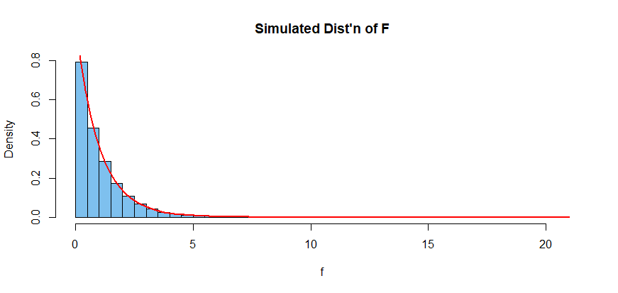
Each random scrambling during the permutation test had a slightly different number of denominator degrees of freedom. So the simulated F-distribution is a mixture of F-distributions. Nevertheless, we notice that the simulated distribution of F is not far from the distribution $\mathsf{F}(2,48)$ of Welch's ANOVA.

hist(f, br=40, prob=T, col="skyblue2", 
   main="Simulated Dist'n of F")
  curve(df(x, 2, 48), add=T, lwd=2, col="red")

Notes: (1) The Welch ANOVA has become popular relatively recently. So its behavior for nonnormal data is perhaps not fully understood. In my own experience, the Welch ANOVA has worked well for sample sizes around two dozen, even if data are discrete, and there are a few outliers. (2) As shown above, the permutation test is programmed in a way that is easy to write, and I hope to understand. However, this code runs slowly. I would not run it again for every one of your Likert items. If you have doubts about the Welch ANOVA in a few specific cases, you might try permutation tests for the relevant data.