Analysis of interaction with multiple levels in each factor (emmeans in mixed model)

Question

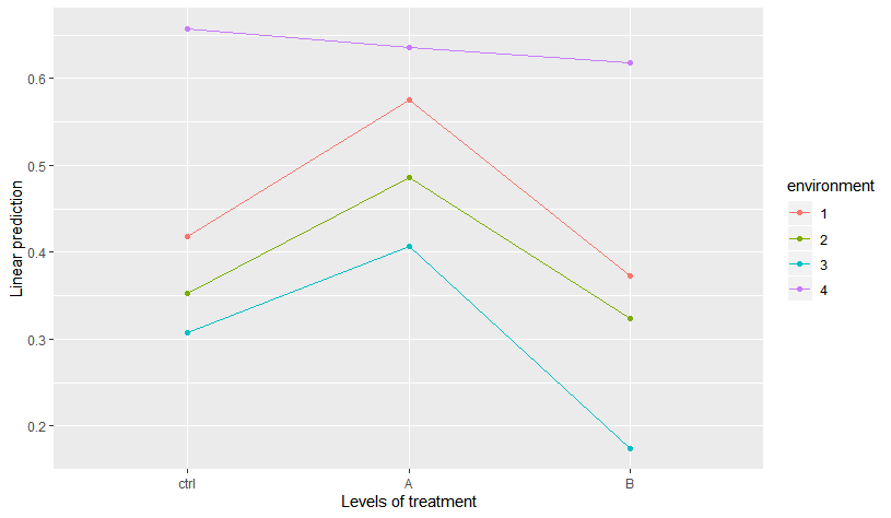
I ran an experiment with treatment (3 levels: ctrl, A, B) as a between-subject factor and environment (4 levels: 1, 2, 3, 4) as a within subject factor. I have grounds to believe there should be an interaction between these two.

To analyze the data, I am using lmer class in R:

> m1 <- lmer(Y ~ environment * treatment + (1 | subjID), data = d)
> anova(m1)

Type III Analysis of Variance Table with Satterthwaite's method
                      Sum Sq Mean Sq NumDF DenDF F value    Pr(>F)    
environment           7.6606 2.55353     3   360 51.2823 < 2.2e-16 ***
treatment             0.9647 0.48237     2   120  9.6874 0.0001258 ***
environment:treatment 0.7344 0.12240     6   360  2.4582 0.0241984 *  
---
Signif. codes:  0 ‘***’ 0.001 ‘**’ 0.01 ‘*’ 0.05 ‘.’ 0.1 ‘ ’ 1

So, indeed, there seems to be a significant interaction. Moreover, using emmeans it is easy to visualize this interaction is triggered mainly by the different effect of treatment in environment 4:

> emmip(m1, environment ~ treatment)

I would like to do analysis of contrasts to show this statistically. I know how to do pairwise comparisons within each level of environment, which is easy:

> emmeans(m1, list(pairwise ~ treatment | environment), adjust = "holm", 
          lmer.df = "satterthwaite")

$`emmeans of treatment | environment`
environment = 1:
 treatment    emmean         SE     df   lower.CL  upper.CL
 ctrl      0.4180488 0.03909552 426.06 0.34120468 0.4948929
 A         0.5754762 0.03862729 426.06 0.49955241 0.6514000
 B         0.3735000 0.03958120 426.06 0.29570128 0.4512987

environment = 2:
 treatment    emmean         SE     df   lower.CL  upper.CL
 ctrl      0.3526829 0.03909552 426.06 0.27583882 0.4295270
 A         0.4866667 0.03862729 426.06 0.41074289 0.5625904
 B         0.3240000 0.03958120 426.06 0.24620128 0.4017987

environment = 3:
 treatment    emmean         SE     df   lower.CL  upper.CL
 ctrl      0.3078049 0.03909552 426.06 0.23096077 0.3846490
 A         0.4069048 0.03862729 426.06 0.33098098 0.4828285
 B         0.1745000 0.03958120 426.06 0.09670128 0.2522987

environment = 4:
 treatment    emmean         SE     df   lower.CL  upper.CL
 ctrl      0.6570732 0.03909552 426.06 0.58022907 0.7339173
 A         0.6352381 0.03862729 426.06 0.55931431 0.7111619
 B         0.6185000 0.03958120 426.06 0.54070128 0.6962987

Degrees-of-freedom method: satterthwaite 
Confidence level used: 0.95 

$`pairwise differences of treatment | environment`
environment = 1:
 contrast    estimate         SE     df t.ratio p.value
 ctrl - A -0.15742741 0.05495933 426.06  -2.864  0.0088
 ctrl - B  0.04454878 0.05563390 426.06   0.801  0.4237
 A - B     0.20197619 0.05530587 426.06   3.652  0.0009

environment = 2:
 contrast    estimate         SE     df t.ratio p.value
 ctrl - A -0.13398374 0.05495933 426.06  -2.438  0.0304
 ctrl - B  0.02868293 0.05563390 426.06   0.516  0.6064
 A - B     0.16266667 0.05530587 426.06   2.941  0.0103

environment = 3:
 contrast    estimate         SE     df t.ratio p.value
 ctrl - A -0.09909988 0.05495933 426.06  -1.803  0.0721
 ctrl - B  0.13330488 0.05563390 426.06   2.396  0.0340
 A - B     0.23240476 0.05530587 426.06   4.202  0.0001

environment = 4:
 contrast    estimate         SE     df t.ratio p.value
 ctrl - A  0.02183508 0.05495933 426.06   0.397  1.0000
 ctrl - B  0.03857317 0.05563390 426.06   0.693  1.0000
 A - B     0.01673810 0.05530587 426.06   0.303  1.0000

P value adjustment: holm method for 3 tests 

but I would like first to say something like "the effect of treatment on Y is different in environment 4 than in the other environments" (basically to test the clear pattern in the figure above). So, what I am struggling with is how to test the general effect of treatment within each level of environment and how to test if these effects differ across environments.

Moreover, I would then like to test if the "general" interaction is a result of a different effect of treatment A in different environments or the result of a different effect of treatment B in different environments (or both). I can do this easily if I run new models with just subsets of the data but I bet there should be an easy way to all this with the original model.

Answer 1

I'd suggest looking at interaction contrasts; something like this:

emm <- emmeans(m1, ~ treatment * environment)
contrast(emm, "eff", by = "environment")           # show the treatment effects
contrast(emm, interaction = c("eff", "pairwise"))  # compare the treat effs

This will display, and then compare, the treatment effects (means minus grand means) between environments. (From the graph, the treatment effects are all small for environment 4, whereas for the other three, the treatment effects are negative for treatments ctrl and B and positive for treatment A.)

You might want something besides "pairwise" so as to have fewer comparisons to look at; e.g., "consec" will restrict to just consecutive levels of environment.

Addendum

Here's a more compact approach: First get the effects, then construct a contrast comparing the average of the first 3 environments with the last:

emm <- emmeans(m1, ~ treatment * environment)   # as before
trt.effs <- contrast(emm, "eff", by = "environment", name = "trt.eff")

At this point we have two "factors" -- environment and trt.eff; the latter has levels ctrl effect, A effect, and B effect. Now let's contrast these:

icons <- contrast(trt.effs, list(`4.vs.123` = c(-1,-1,-1,3)/3), 
                  by = "trt.eff")
summary(icons, by = NULL, adjust = "mvt")

These are manually constructed interaction contrasts -- contrasts of contrasts. You could just display icons as the three different by groups with one contrast each. But if summarized as shown with by = NULL, we combine them into one family and apply a multivariate t multiplicity adjustment for the family of three tests.

Answer 2

With regard to the first part of your question, i.e.,

how to test the general effect of treatment within each level of environment

You would need to specify the appropriate contrasts to achieve this. The emmeans package seems to offer the possibility to define your own contrasts function; for more info, see here.

With regard to the second part, i.e.,

how to test if these effects differ across environments

if I understand correctly what you mean, I would say that this is the overall interaction effect that you got from the anova() function.