Monte Carlo simulation for the log-normal distribution

Question

Consider $X$ that follows a log-normal distribution with parameters $\mu=1$ and $\sigma=1$. The moments are known: $m_n=E[X^n]=e^{n+n^2/2}$. For example, $m_{10}=e^{60}$ (of the order of $10^{26}$). I simulate samples of $X^{10}$ in Mathematica of length $1,000,000$, and I notice that the mean values of such samples are always less than $e^{60}$:

Mean[RandomVariate[LogNormalDistribution[1, 1], 1000000]^10] < Exp[60]
(* Comment: The output seems always to be True. *)

Why is Monte Carlo simulation not working with the log-normal distribution? The tails of the distribution (the extreme values) should be the problem, I think. Is there a modification of the Monte Carlo simulation to tackle this problem?

Answer 1

From your expression above for $m_n$, you can derive the following:

$$P[X^n > m_n] = 1 - \Phi(n/2)$$

For $n=10$, that's less than 0.3 per million, so the vast majority of samples will be smaller than $m_n$ (and it's not unusual to not have a single sample out of 1 million turn out to be larger than $m_n$). It's the rare but very large values that pull up the moment, as you mention, and it gets more evident for larger moments.

One relatively simple method for improving a Monte Carlo method that depends critically on rare events is to use importance sampling and "tweak" the distribution to make those events more likely, and then weigh our samples to get back to the distribution we're actually trying to sample from. One such approach is called exponential twisting (or tilting). For example, for a normal distribution $Y\sim \mathcal{N}(\mu,\sigma^2)$, consider the twisted random variable:

$$Y_\theta \sim \mathcal{N}(\mu + \theta\sigma^2,\sigma^2)$$

For some function $f$ of interest, you can show that:

$$E(f(Y)) = E_{\theta}\left[f(Y)p(Y)/p_{\theta}(Y)\right]=E_{\theta}\left[f(Y)e^{(\mu-Y)\theta+\sigma^2\theta^2/2}\right]$$

The expectation $E$ is taken with respect to the distribution of $Y$, while $E_{\theta}$ is with respect to that of $Y_{\theta}$. The parameter $\theta$ can be tuned depending on the problem at hand (e.g. which events we need to make more likely), and $\theta = 0$ corresponds to the regular MC method.

The above identity means that you can then estimate the expectation of interest on the left by Monte Carlo like this:

1. Draw $Y_i \sim \mathcal{N}(\mu + \theta\sigma^2,\sigma^2)$
2. Compute the weighted sample average $\frac{1}{M}\sum_{i=1}^M f(Y_i) e^{(\mu-Y_i)\theta+\sigma^2\theta^2/2}$

For your specific problem, you would take $\mu = 10$, $\sigma^2 = 100$ and $f(x) = e^x$.

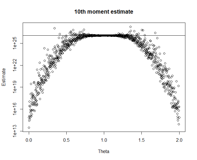
For a range of values of $\theta$, sampling only 1000 $Y_i$'s for each value, I obtain the following estimates (the horizontal line is the exact value):

We see that the regular MC method ($\theta=0$) performs poorly, and that values near $\theta=1$ produce a result much closer to the true value.

Obviously, this is a somewhat contrived example: if I simply take $\theta = 1$, then $Y_i = e^{\mu+\sigma^2/2}$ for all $i$, and I get the exact result with no sampling variation, which we already knew from the beginning. The method can still be used in other situations where a closed-form solution or other efficient numerical approximation does not exist.