Residual plot from a logistic regression

Question

Reposting from here

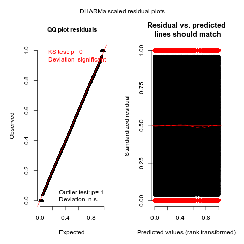
I am implementing a two-stage logistic regression customer acquisition model and want to understand the peculiar pattern I observe in the residuals from the DHARMa R package.

The first stage model is a probit model

selection_model <- glm(I(acquired > 0) ~ m * b + l + w + f,
                       data = aggregate_df,
                       family = binomial(link = "probit"))

Then I add in the inverse mills ratio like so:

aggregate_df$IMR = dnorm(selection_model$linear.predictors)/pnorm(selection_model$linear.predictors)

The second stage model shares the same predictors except that the inverse mills ratio is also added as a predictor. Also, I am interested in looking at those customers who have given a total sales of more than X. This is captured in a binary indicator variable I(dollar_sales > X), which is the outcome I model in the second stage.

model_logit <- glm(I(dollar_sales > X) ~ IMR + m * b + l + w + f + 
                                         I(f^2) + I(l^2),
                   data = aggregate_df,
                   family = binomial(link = "logit"))

I then plot the residuals of this model using the DHARMa package like so:

simulated_residuals = DHARMa::simulateResiduals(model_logit, n = 50)
plot(simulated_residuals)

I have the following questions:

1. Why are there two disjoint blobs at the bottom and top of the QQ plot? Is this a cause of concern (as the KS test indicates)?
2. The residual vs predicted plot seems okay, barring the outliers. Is this also expected behavior