0
$\begingroup$

I have a data set about 5,699 PhD students. The first column called "Year" is how many years it took for candidate to graduate with a Ph.D (1, 2,...14), the second column "Uni" is which university the student received the PhD, and the third column "Res" is residency of subject (permanent or temporary)

> head(mydata)
   Year     Uni       Res
1    1 Berkeley Permanent
2    1 Berkeley Permanent
3    1 Berkeley Permanent
4    1 Berkeley Permanent
5    1 Berkeley Permanent
6    1 Berkeley Permanent

I wish to see if there is a significant difference in the number of years it took for PhD students to graduate by residency. I'm assuming I must perform a two sample t-test or a two sample z-test. I know that one performs a z-test if the standard deviation of the population is known, and a t-test if it is not known. However, I have no information on whether these 5,699 students form a population or if they are samples from a larger population. Since I am not sure, should I perform the two sample t-test? Does it even matter since my degrees of freedom are so large?

One of the assumptions of the two sample t-test and the two sample z-test is that the data must be normally distributed. Does this mean I have check if the number of years to graduate is normal for each group (permanent, temporary) or do I combine the data and check to see if the years to graduation is normal? What kind of tests do I use to check for normality in this case? Are there other assumptions I should be aware about?

$\endgroup$
3
  • 2
    $\begingroup$ What happens when a student drops out? $\endgroup$
    – AdamO
    Commented Oct 10, 2019 at 22:01
  • $\begingroup$ I'll repeat my comment from the duplicated question: if your dependent variable, years, takes on few and discrete values, you might need to use a test more appropriate for ordinal data. I can imagine this data might be quite skewed, and of course bound by 1 on the left. $\endgroup$ Commented Oct 10, 2019 at 22:15
  • $\begingroup$ This sounds like it might be better handled by survival analysis, perhaps discrete-time given the small number of distinct event (graduation) times. Dropping out could be considered a competing event, handling the important point made by @AdamO in another comment. Normality would no longer be an issue either. $\endgroup$
    – EdM
    Commented Oct 11, 2019 at 0:36

2 Answers 2

3
$\begingroup$

There are a few parts of your question I'd like to address:

I have no information on whether these 5,699 students form a population or if they are samples from a larger population.

They almost certainly should be considered a sample from a population. This is true for almost every dataset. Ask yourself this: Do those 5,699 students make up the entire population of graduate students in the world, throughout all time? If not, then they aren't the population. Even if it were, the entire point of statistical inference is that you do not have access to the population's data. If you did, you would simply compute the average years-to-graduation in each group and conclude, with 100% certainty, that "yes, they are different." There would be no need for a statistical test.

should I perform the two sample t-test? Does it even matter since my degrees of freedom are so large?

It's true that, with a large enough sample, the t-test and z-test are largely the same. I suspect that with a sample of your size the difference would be very small (unless the two groups are very unbalanced). However, I would simply run a t-test because this constitutes a more conservative assumption on the data.

Does this mean I have check if the number of years to graduate is normal for each group (permanent, temporary) or do I combine the data and check to see if the years to graduation is normal?

You would need to check the distribution of years-to-graduate in each group (2 distributions). Although you have a large amount of data and normality may not be a concern, the discreteness of your data (1 year, 2 year, 3 year...) may become an issue. If you prefer to use a numerical test rather than a simple examination of your data, I suggest the Shapiro-Wilk test, which you can perform in R:

shapiro.test(myData)

Where a p-value > 0.05 indicates weak evidence that your data are not normal.

If your data appear to be nastily distributed or fail the Shapiro test, I would recommend a nonparametric alternative to the t-test, the Wilcoxon rank-sum test, also implementable in R.

$\endgroup$
4
  • 1
    $\begingroup$ @AdamO makes a good point: your data may be right-truncated, which means that people who never experience the event of interest (i.e., graduation) are not observed on your data. You are effectively testing the "time to graduation" among only students who have graduated! Consider a school that has a 99% dropout rate but whose remaining population graduate within 4 years. Would you really consider their average time-to-graduation to be 4 years when there are so many people who never graduate at all? $\endgroup$
    – G. Vece
    Commented Oct 10, 2019 at 22:10
  • $\begingroup$ Ultimately, you may not have access to a "better" dataset that will allow you to address this issue; however, it will be a major weakness of your analysis if not accounted for. $\endgroup$
    – G. Vece
    Commented Oct 10, 2019 at 22:12
  • $\begingroup$ (+1) Especially, for mention of @AdamO's comment and (even though probably not necessary) the Wilcoxon rank sum test. $\endgroup$
    – BruceET
    Commented Oct 10, 2019 at 22:33
  • $\begingroup$ Good answer. The only thing I would change is that I don't recommend using Shapiro test ( or any other test ) for this kind of purpose. One objection is theoretical:. That now you're making one test contingent on the results of another test. So how does one interpret the p-value? Also, practically, if you have a large sample size, you might be likely to get a significant result even if the data are close enough to normal to yield reasonable results for the e.g. t-test. $\endgroup$ Commented Oct 10, 2019 at 23:48
1
$\begingroup$

Exact vs. estimated population variances. I suppose you do not know the exact values of $\sigma_P^2$ and $\sigma_T^2,$ and that you would use respective sample variances $S_P^2$ and $S_T^2$ as estimates. Then technically speaking, you have no choice but to do a t test. (If you do a z test with estimated variances, you are really doing an approximate t test, depending that the large degrees of freedom with provide a good approximation.)

Equal vs. unequal population variances. I see no basis for assuming that $\sigma_P^2 = \sigma_T^2,$ so your test should not assume equality. If you do a two-sample t test, then you should use the Welch (not pooled) version. (In R, the Welch version is the default: you would have to use parameter var.eq=T in the t.test procedure to select the pooled version.) If you do an approximate z test, then be sure to supply proper estimates for $\sigma_P^2$ and $\sigma_T^2$ in the denominator of the test statistic.

Checking for normal data. With several thousand in each group (P and T), the t test should be sufficiently robust against mild non-normality that you would have no qualms about doing the t test. If individual boxplots of P and T groups separately show only a few moderate outliers, and show no evidence of extreme skewness, that would indicate that using the Welch t test is OK. (With data values between 1 and 14, I would not expect difficulties.)

As a technical matter it is the residuals that need to be normal for a precisely accurate t test. So if it is important to check for normality, you should look at P and T groups separately. (However, formal normality tests, such as Shapiro-Wilk, may be far too aggressive in detecting harmless departures from normality. See Comment of @SalMangiafico and my Addendum.)

Summary. Without knowing whether your data can be considered as a valid random sample from the two groups, without seeing actual data data values, and just guessing from academic experience about PhD finishing times, my guess is that you should use a Welch two-sample t test.


Addendum. (Prompted by various comments.)

Suppose both P and T samples have means somewhat above 4 years, as for the fake data below. I am not suggesting that these data are similar to yours, but they do illustrate uses of various possibly relevant methods.

set.seed(2019)
prm = rbinom(3000, 9, .35) + 1
tmp = rbinom(2700, 9, .4) + 1

summary(prm); sd(prm)
 Min. 1st Qu.  Median    Mean 3rd Qu.    Max. 
1.000   3.000   4.000   4.133   5.000   9.000 
[1] 1.423371
summary(tmp); sd(tmp)
 Min. 1st Qu.  Median    Mean 3rd Qu.    Max. 
1.000   4.000   5.000   4.566   6.000   9.000 
[1] 1.480406

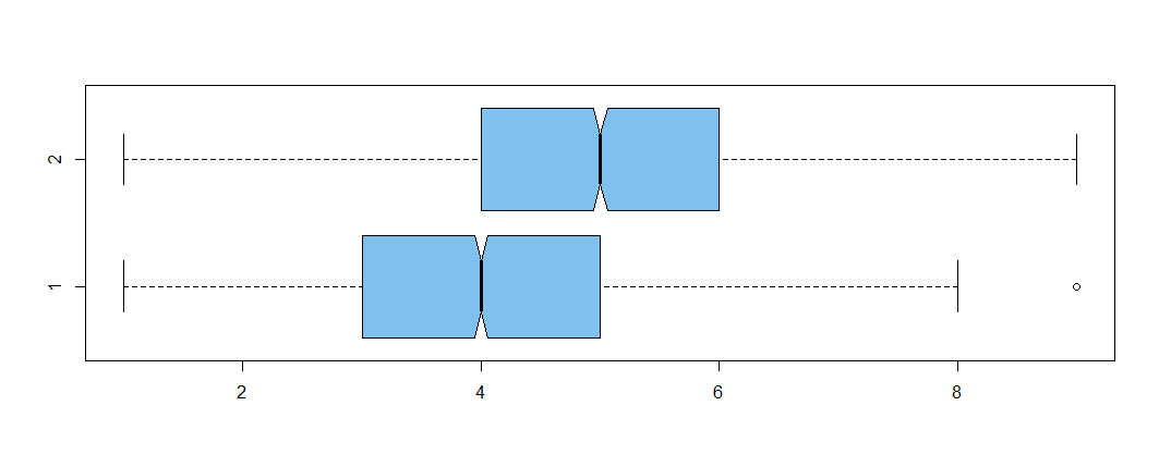
boxplot(prm,tmp, col="skyblue2", horizontal=T, notch=T)
enter image description here

The 'notches' in the sides of the boxes show nonparametric confidence intervals calibrated so that non-overlapping CIs for two groups suggests a significant difference in locations at the 5% level.

My (essentially binomial) data in Group P look nearly normal in a histogram (with 'best-fitting' normal density). However, the Shapiro-Wilk test strongly rejects their normality---possibly, mostly just because all values are integers. See Note. [Similar results for the data in Group T are not shown.]

enter image description here

shapiro.test(prm)$p.val
[1] 1.315475e-29

Both the two-sample Welch t test and the (nonparametric) two-sample Wilcoxon signed-rank test strongly reject the null hypothesis that the two populations the same. With such large samples, you have good power to detect even fairly small differences in location between time until PhD for P and T groups. In the figure, the intervals are far from overlapping.

t.test(prm, tmp)

         Welch Two Sample t-test

data:  prm and tmp
t = -11.236, df = 5581.4, p-value < 2.2e-16   # df=5698 for 'pooled'
alternative hypothesis: 
  true difference in means is not equal to 0
95 percent confidence interval:
  -0.5088930 -0.3576996
sample estimates:
mean of x mean of y 
 4.133000  4.566296 

wilcox.test(prm, tmp, conf.int=T)

        Wilcoxon rank sum test with continuity correction

data:  prm and tmp
W = 3371100, p-value < 2.2e-16
alternative hypothesis: true location shift is not equal to 0
95 percent confidence interval:
 -9.999792e-01 -3.957901e-05
sample estimates:
difference in location 
         -2.474458e-05 

Note: In the experiment below, the Shapiro-Wilk test does not recognize normal data rounded to integers as being normal.

z = rnorm(3000, 5, 1); shapiro.test(z)$p.val
[1] 0.583755                # Accept null: data normal
rz = round(z); shapiro.test(rz)$p.val
[1] 5.377162e-37            # Reject null: rounded data not normal
$\endgroup$

Your Answer

By clicking “Post Your Answer”, you agree to our terms of service and acknowledge you have read our privacy policy.

Not the answer you're looking for? Browse other questions tagged or ask your own question.