Why would predicted values be normally-distributed when the actual values are uniform?

Question

I'm building a supervised learning model where the target variable is a uniformly-distributed continuous value ranging from 0-1 (originally a rank value from 1-38000, then scaled down to 0-1). The 20 predictor variables are a mix of continuous and categorical variables, with no more than 6 levels for the latter. But when I apply various modeling techniques to the data (including regression, random forest, MARS, neural nets) using R, the predicted values for every model are shaped like a bell curve.

What could cause the fitted values (bell shape) to be so consistently different from the actual ones (uniform shape)? And is there any way to force these models to produce a more uniformly-shaped prediction?

Answer 1

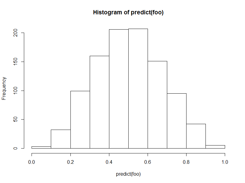
First, to address the issue of bell-shaped predictive values. This will be a heuristic explanation, to say the least. Let's take a linear regression as our "example" case. If you think of the predictor variables as being drawn from some 20+ - dimensional probability distribution (more on the "+" later), a prediction from a linear regression can be thought of as a weighted average of 20+ random variables... the distribution of which, under a wide range of conditions, will tend towards Normality as the number of random variables goes up. Hence the bell-shaped curve.

The "+" is present because, from a numerical standpoint, a categorical variable with 6 levels is equivalent to 6 binary variables (which, obviously, are not independent.) Note I'm not claiming that these 6 binary variables contribute to the asymptotic Normal distribution to the same degree as a continuous variable would.

Insofar as other methodologies all have a "weighted average" flavor to them, something similar will occur, though mediated by the actual calculations involved. Here's an example using random forests; I have 10 predictors, independently distributed $U(0,1)$, and the target variable $y$ is the normalized rank of the sum of the square roots of the 10 predictors (so $y$ is in (0,1]).

U <- as.data.frame(matrix(runif(10000),1000))
y <- rowSums(sqrt(U))
U$y <- rank(y)/length(y)

foo <- randomForest(y~V1+V2+V3+V4+V5+V6+V7+V8+V9+V10, mtry=4, data=U)
hist(predict(foo))

As you can see, the bell-shaped histogram of the predicted values occurs in other contexts than yours.

Second, converting to a more uniformly-shaped prediction. One way would be to rank the predicted values from 1-38000, then scale down to 0-1, just as with the original rank-valued target variable.

Here's what happens when we continue the above example in this vein:

> u.predict <- rank(predict(foo))/length(predict(foo))
> mean((u.predict-U$y)^2)
[1] 0.007450796

> mean((predict(foo)-U$y)^2)
[1] 0.01875836

The mean squared error of the ranked predictions has decreased by a factor of roughly 2.5 relative to the "raw" predictions. My guess as to why this works, which I admit surprised me, is that the original variable is a normalized rank, not a true interval-valued variable (i.e., 0.002 is not 2 times 0.001, really,) and the ranked predictions are in a way correcting for the fact that the estimation procedures are all assuming that they are.