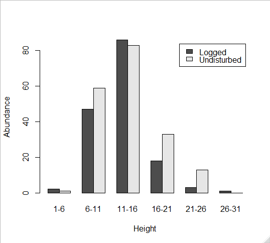
For an effective ad hoc test, I suggest you use
height categories 'Below 16' and 'Above 16' for
each type of forest. This will result in at $2 \times 2$
table with sufficiently large counts to use a
chi-squared test.
TBL = rbind(c(135,22), c(143,46))
cq.out = chisq.test(TBL);  cq.out

   Pearson's Chi-squared test
   with Yates' continuity correction

data:  TBL
X-squared = 5.1553, df = 1, p-value = 0.02318
Then compare observed and expected counts.
cq.out$obs
     [,1] [,2]
[1,]  135   22
[2,]  143   46
cq.out$exp
         [,1]     [,2]
[1,] 126.1445 30.85549
[2,] 151.8555 37.14451

cq.out$res
           [,1]      [,2]
[1,]  0.7884579 -1.594213
[2,] -0.7186169  1.452999
Under the null hypothesis that type of forest and
height categories of trees are independent, you would expect
around 31 'tall' trees in the logged forest and 37 in the
undisturbed forest.
In fact, respective observed counts of tall trees are 22 and 46. These
discrepancies are the largest contributors to the fact
that the chi-squared statistic is significantly large.
The Pearson residuals are the signed square roots
of the components $r_{ij}^2=\frac{(X_{ij}-E_{ij})^2}{E_{ij}}.$
If the chi-squared test rejects in a 2-by-2 table, then the cells where absolute values $|r_{ij}|$ of
residuals are largest often point the way to important departures from the null hypothesis.
But be careful, you should not go so far as to claim
that trees in the undisturbed forest are generally taller. The median heights of trees is about the same (13.5 ft) in both.
Also, mean heights are about the same (near 13 ft) in both.
If you don't have the original heights, then you could roughly reclaim them by using interval midpoints:
x = rep(seq(3.5,28.5,by=5), c(2,47,86,18,3,1))
y = rep(seq(3.5,28.5,by=5), c(1,59,83,33,13,0))
Summaries of these approximate heights are
similar for the two forests, as follows:
summary(x)
    Min. 1st Qu.  Median    Mean 3rd Qu.    Max.
    3.50    8.50   13.50   12.74   13.50   28.50
summary(y)
    Min. 1st Qu.  Median    Mean 3rd Qu.    Max.
    3.50    8.50   13.50   13.45   13.50   23.50
Also, a two-sample t.test on the approximate heights does not show significance at the 5% level.
t.test(x,y)$p.val
[1] 0.1092758
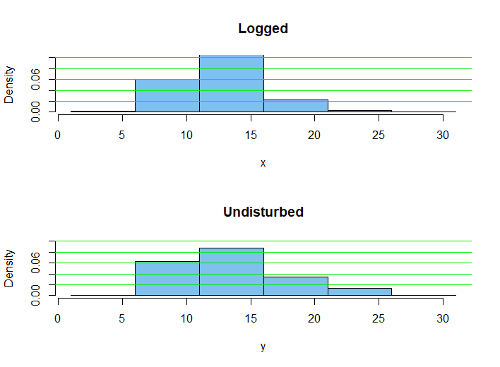
Addendum: Density histograms based on height categories.

R code for histogram:
cutp = seq(1,31,by=5)
par(mfrow=c(2,1))
 hist(x, prob=2, br=cutp, ylim=c(0,.1), col="skyblue2", main="Logged")
  abline(h=seq(.02, .1, by=.02), col="green2")
 hist(y, prob=2, br=cutp, ylim=c(0,.1), col="skyblue2", main="Undisturbed")
  abline(h=seq(.02,. 1, by=.02), col="green2")
par(mfrow=c(1,1))
Addendum: If you want a way to focus just on the tallest
trees, you can compare the proportion of them in the logged
forest with the proportion of them in the undisturbed
forest. That's $22/157$ vs. $46/189.$ Again, you get a P-value
about 2% (as for the chi-squared test), but without discussing
observed and expected counts:
prop.test(c(22,46), c(157,189))

        2-sample test for equality of proportions
        with continuity correction

data:  c(22, 46) out of c(157, 189)
X-squared = 5.1553, df = 1, p-value = 0.02318
alternative hypothesis: two.sided
95 percent confidence interval:
 -0.19088789 -0.01562982
sample estimates:
   prop 1    prop 2
0.1401274 0.2433862


