ARIMA forecasts with autocorrelated residuals

Question

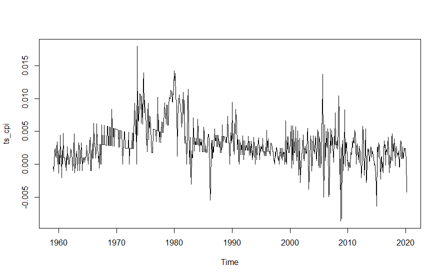
I have a time series on consumer price index (CPI) and want to forecast inflation which is in my case the first difference of the log of CPI: π_t=Log(P_t) - Log(P_t-1). This is the time series:

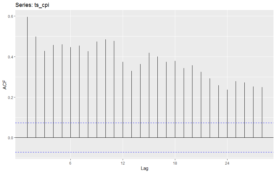
The ACF of the series decreases slowly as the lag increases (trend?) and a typical “scalloped” shape is also observable (seasonality?).

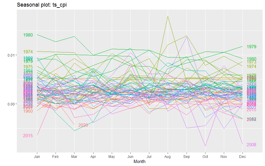
From my perspective there is no clear evidence for seasonality according to the seasonalityplot. However in the final ARIMA model when applying auto.arima seasonality is taken into account.

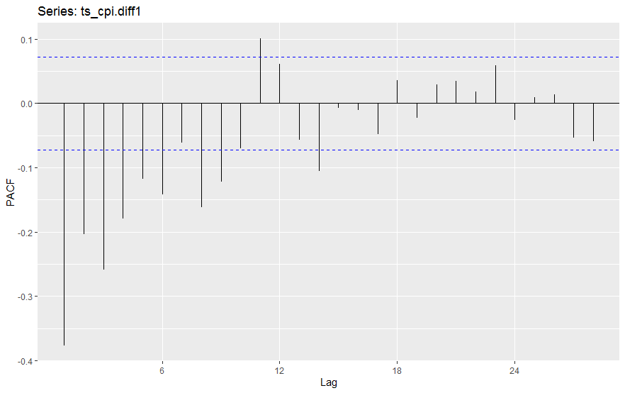
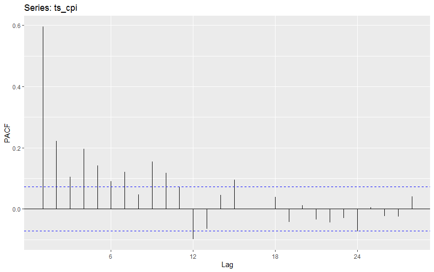
Both the ADF test and KPSS test verify that this time series is nonstationary. Ndiffs() suggest to use d=1. the ADF test and KPSS test verify that the first diff series is stationary. The ACF and PACF plots are the following: 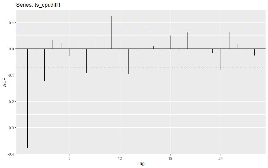Applying the auto.arima function yields the following results:

Series: ts_cpi 
ARIMA(3,1,1)(0,0,2)[12] 

Coefficients:
       ar1      ar2      ar3      ma1     sma1     sma2
      0.1740  -0.0102  -0.1190  -0.8345  -0.0764  -0.1181
s.e.  0.0466   0.0415   0.0414   0.0306   0.0370   0.0352

sigma^2 estimated as 4.914e-06:  log likelihood=3442.04
AIC=-6870.08   AICc=-6869.93   BIC=-6837.9

Training set error measures:
                   ME        RMSE         MAE           
Training set 4.863658e-06 0.002206118 0.001545581  

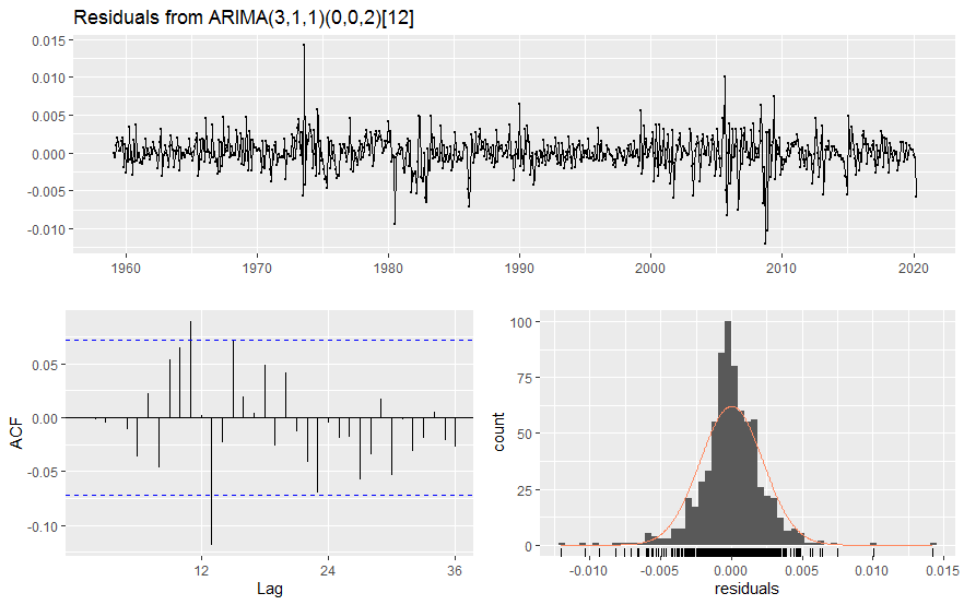
The Ljung-Box test indicates that the residuals are autocorrelated (24lags):

Ljung-Box test

data:  Residuals from ARIMA(3,1,1)(0,0,2)[12]
Q* = 38.23, df = 18, p-value = 0.003611

Model df: 6.   Total lags used: 24

How can i proceed in order to have uncorrelated residuals and thus stable forecast estimations? Should i manually add more lags to the ARIMA model or make use of heteroskedastic robust errors?

Answer 1

As you already see in your data, inflation is a highly persistent, non-stationary, process.

(The sample ACF of your inflation series is probably significant at all lags, up to the size of your sample.)

As it does not make sense to speak of forecast for non-stationary series, one typically performs forecast for change in inflation, i.e. its first-difference.

Taking the first-difference loses information on the mean of the series. If your data is from an advanced economy, this is not an issue. The sample mean of the inflation series would typically be very close to the central bank's announced inflation target (you should verify this).

Fit ARMA models to the first-difference of inflation series and select by comparing pseudo-out of sample forecast mean square errors. Start with simple AR models, as they have the most economic meaning in this context. You can already notice the standard OLS/conditional MLE estimate of the AR(1) parameter is going to be negative, as it should be---this reflects the central bank's attempt at stabilizing inflation when it over/under shoots the target. Yes, use robust standard errors to compute MSFE if applicable.