Change of variables in pdf

Question

I have the joint pdf$$f(x_1,x_2)=x_1e^{-x_1(1+x_2)}I_{(0,\infty)}(x_1)I_{(0,\infty)}(x_2)$$and have to derive the joint pdf of $$Y_1=e^{-X_1}\qquad\text{ and }\quad Y_2=e^{-X_1X_2}$$ I set $x_1=-\ln(y_1)$ and $x_2=\ln(y_2)/\ln(y_1)$. When I plug these transforms into $f(x_1,x_2)$ and multiply with the absolute determinant of the Jacobian $|\det(J)|=1/(y_1y_2\ln(y_2))$, I get a negative result. Where did I make a mistake?

Answer 1

Let's first explore how much progress we can make without trying to solve for the x's in terms of the y's and by avoiding a direct calculation of the Jacobian (according to the Principle of Mathematical Laziness).

From

$$\mathrm{d}y_1 = -e^{-x_1}\mathrm{d}x_1$$

and

$$\mathrm{d}y_2 = -e^{-x_1x_2}\left(x_2\mathrm{d}x_1 + x_1\mathrm{d}x_2\right),$$

both computed using elementary rules of differentiation, notice that

$$\mathrm{d}y_1\wedge \mathrm{d}y_2 = \left(-e^{-x_1}\right)\left(-e^{-x_1x_2}\right)\left(x_1 \mathrm{d}x_1\wedge\mathrm{d}x_2\right) = x_1e^{-x_1(1+x_2)}\mathrm{d}x_1\wedge\mathrm{d}x_2,$$

which we may use in a first step towards transforming the probability element:

$$f_{X_1,X_2}(x_1,x_2)\mathrm{d}x_1\mathrm{d}x_2 = \mathcal{I}_{(0,\infty)}(x_1)\mathcal{I}_{(0,\infty)}(x_2)\,\mathrm{d}y_1\mathrm{d}y_2.\tag{*}$$

(This is a bit of an abuse of notation: we must think of the $x_i$ on the right hand side as being functions of the $y_i,$ whereas on the left hand side the $x_i$ are just variables.)

It remains only to re-express the indicator functions in terms of $(y_1,y_2).$ Since $0 \lt x_1 \lt \infty,$

$$1 = e^{-0} \gt e^{-x_1} = y_1 \gt e^{-\infty} = 0$$

and

$$1 = e^{-0} \gt e^{-x_1x_2} = y_2 \gt e^{-\infty(\infty)} = 0.$$

Thus $(*)$ becomes

$$f_{X_1,X_2}(x_1,x_2)\mathrm{d}x_1\mathrm{d}x_2 = \mathcal{I}_{(0,1)}(y_1)\mathcal{I}_{(0,1)}(y_2)\,\mathrm{d}y_1\mathrm{d}y_2$$

from which we can read off the density as

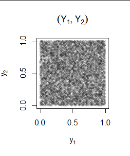
$$f_{Y_1,Y_2}(y_1,y_2) = \mathcal{I}_{(0,1)}(y_1)\mathcal{I}_{(0,1)}(y_2).$$

This is, of course, the uniform density on the unit square $(0,1)^2.$ As a check, let's plot some simulated values of $(Y_1,Y_2).$ In R this can be carried out as

n <- 1e4
x1 <- rexp(n)
x2 <- rexp(n, x1)
y1 <- exp(-x1)
y2 <- exp(-x1*x2)
plot(y1, y2, asp=1, xaxp=c(0, 1, 2), yaxp=c(0, 1, 2),
     pch=19, cex=1/2, col="#00000010", 
     main=expression(group("(", list(Y[1], Y[2]), ")")),
     xlab=expression(y[1]), ylab=expression(y[2]))

(This works because $X_1$ has an exponential distribution and, conditional on $X_1,$ $X_2$ has an exponential distribution with rate $X_1.$) The plot of the y-values indeed fills the unit square uniformly (up to expected statistical fluctuations):