Monte carlo results becomes more skewed with more sampling

Question

I'm running a monte carlo simulation of a financial instrument, and I'm trying to understand why the final balance of each simulation gives me a skewed distribution rather than a normal distribution (given that I'm sampling out of a normal distribution using np.random.normal).

I assume average monthly return of 1%, standard deviation of 4 and projecting for 60 months. My method is to sample from a normal distribution using np.random.normal and create an array out of that. Then I take a starting balance and multiply that over each element and create a list. I append 500 of these simulations to a dataframe:

df = pd.DataFrame()
for i in range(1, 501): #500 simulations
    pct = np.random.normal(loc = 1, scale = 4, size = 60) #mean 1%, std 4%, 60 month period
    df['Simulation_' + str(i)] = balance_updater(100000, pct)

where the function balance_updater creates a list that documents every iteration (in this case, starting balance = 100000), coded as the following:

def balance_updater(starting_balance, pct):
    balance = starting_balance
    balance_list = []
    for i in range(len(pct)):
        balance = (balance + balance * pct[i] / 100).round(2)
        balance_list.append(balance)
    return balance_list

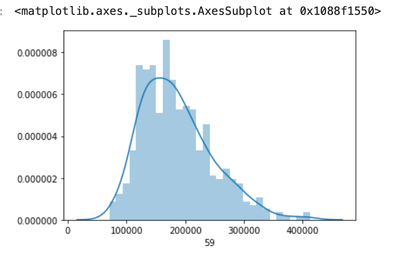
Then when I plot via: sns.distplot(df.iloc[-1, bins=30) #Plot final balances only

This is the resulted graph.

I expected this to be normally distributed but we can see it slightly skewed to the right.

What puzzles me more is that if I were to project for a longer period of time (let's say 30 years = 180 months) the results become even more skewed:

I'm trying to understand why a longer projected period produces a more skewed graph, which violates my understanding of the central limit theorem with more sampling (360 vs 60).

Thank you.

Answer 1

It seems that you take the product of normal distributed variables $X_i \sim N(\mu = 1.01, \sigma = 0.04)$. This is different from a sum of normal distributed variables, for which it would be reasonable to expect that you get a normal distributed variable.

$$Y_{total} = \prod_{i=1}^n(X_i)$$

But you can end up with a sum term by rewriting the above as:

$$Y_{total} = \exp \left( \sum_{i=1}^n \log(X_i) \right)$$

The distribution of the term $\sum_{i=1}^n \log(X_i)$ will approach a normal distribution and what you will end up with is a lognormal distributed variable. The logarithm of your balance is distributed as a sum of many variables, which will approach a normal distribution.

To determine the mean and variance of $\sum_{i=1}^n \log(X_i)$ you need to know the mean and variance of $\log(X_i)$. You can do this with the Delta method, although there is also a more precise method. In the computation example below the more precise method is used for generating the curve, but the code also contains the computations for the other methods.

---

example computation

With this R code you can show that the distribution follows a log normal distribution and you can use a normal distribution (using the central limit theorem) to determine it.

### n = number of months being simulated
n = 180

### product of 180 normal distributed variables
fun <- function() {
  prod(rnorm(n,1.01, 0.04))
}

### perform 10 000 times a simulation
x = replicate(10^4, fun())

### plot histogram
hist(x, breaks = seq(0,100,0.3), xlim = c(0,20), freq = FALSE)

### estimate of mu and sigma based on data
mu = mean(test)*n
sig = var(test)^0.5*sqrt(n)

### Delta method
mu = log(1.01)*n
sig = 0.04*sqrt(n)/1.01

### Improved estimate
mu = (log(1.01)-0.5*(0.04/1.01)^2)*n
sig = 0.04*sqrt(n)/1.01

### plot log-normal distribution with estimate of sig and mu
xs = seq(0,20,0.01) 
lines(xs, dlnorm(xs,mu,sig))

---

Skewness dependency on $n$

For increasing $n$ the standard deviation of $\sum_{i=1}^n \log(X_i)$ will increase, and the skewness (being a function of the standard deviation) will increase as well. Intuitively you can see it as the balance changing each month more in the positive direction than the negative direction (in absolute terms, an increase with 1% is more change than a decrease with 1%), so every month you unevenly stretch/skew the balance.