Recently, I watched this video on YouTube on the solution of ode/pde with neural network and it motivated me to write a short code in Keras. Also, I believe the video is referencing this paper found here.
I selected an example ode $$ \frac{\partial^2 x(t)}{\partial t^2} + 14 \frac{\partial x(t)}{\partial t} + 49x(t) = 0 $$
with initial conditions $$ x(0) = 0, \ \frac{\partial x(t)}{\partial t}\rvert_{t=0} = -3 $$
According to the video, if I understand correctly, we let the neural network $\hat{x}(t)$, be the solution of our ode, so $x(t) \approx \hat{x}(t)$
Then, we minimize the ode which is our custom cost function per say. Since, we have initial conditions, I created a step function for individual data point loss:
At, $t=0$: $$ loss_i = \left( \frac{\partial^2 \hat{x}(t_i)}{\partial t^2} + 14 \frac{\partial \hat{x}(t_i)}{\partial t} + 49\hat{x}(t_i) \right)^2 + \left( \frac{\partial \hat{x}(t_i)}{\partial t} + 3 \right)^2 + \left( \hat{x}(t_i) \right)^2 $$
else $$ loss_i = \left( \frac{\partial^2 \hat{x}(t_i)}{\partial t^2} + 14 \frac{\partial \hat{x}(t_i)}{\partial t} + 49\hat{x}(t_i) \right)^2 $$
Then, minimize batch loss $$ \min \frac{1}{b} \sum_{i}^{b} loss_i $$
where $b$ is the batch size in training.
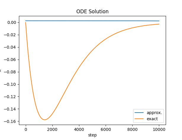
Unfortunately, the network always learns zero. On good evidence, the first and second derivatives are very small - and the $x$ coefficient is very large i.e.: $49$, so the network learns that zero output is a good minimization.
Now there is a chance that I misinterpret the video because I think my code is correct. If someone can shed some light I will truly appreciate it.
Is my cost function correct? Do I need some other transformation?
Update:
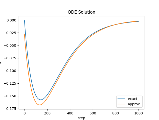
I managed to improve the training by removing the conditional cost function. What was happening was that the the conditions were very infrequent - so the network was not adjusting enough for the initial conditions.
By changing the cost function to the following, now the network has to satisfy the initial condition on every step:
$$ loss_i = \left( \frac{\partial^2 \hat{x}(t_i)}{\partial t^2} + 14 \frac{\partial \hat{x}(t_i)}{\partial t} + 49\hat{x}(t_i) \right)^2 + \left( \frac{\partial \hat{x}(t=0)}{\partial t}\rvert_{t=0} + 3 \right)^2 + \left( \hat{x}(t=0)\rvert_{t=0} \right)^2 $$
The results are not perfect but better. I have not managed to get the loss almost zero. Deep networks have not worked at all, only shallow one with sigmoid and lots of epochs.
Highlight:
I am surprised this works at all since the cost function depends on derivatives of non-trainable parameters. This is interesting to me. I would love to hear some insight.
I would appreciate any input on improving the solution. I have seen a lot of fancy methods but this is the most straight forward. For example, in the referenced paper above - the author uses a trial solution. I do not understand how that works at all.
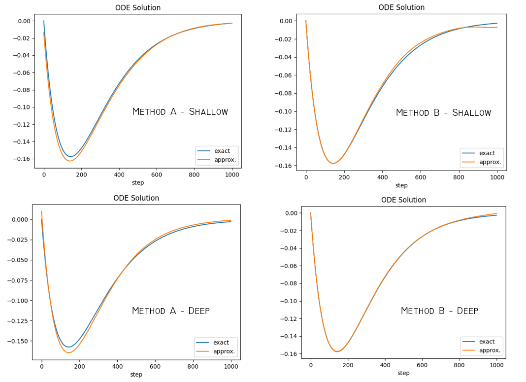
Results:
Method A = method described above
Method B = method described in the accepted answer
Shallow = One layer, 1024 nodes, gaussian activation with $b=2$
Deep = Three layer, 10 nodes each, sigmoid activation in all
The transform method B appears to work better. The other method A, may come in handy as a control method or when boundaries are very difficult to model with a trial function, or when not solving on a rectangular domain.
I think both methods can be improved with better domain sampling instead of random shuffle, for example different sampling for the boundaries and different sampling for points inside the domain where the points are collocated.


