Standard error of estimated covariance

Question

Let $X_1,...,X_n$ and $Y_1,...,Y_n$ be two independent random samples from $\mathcal{N}(\mu, \sigma^2)$ where both $\mu$ and $\sigma$ are unknown parameters.

I estimate their covariance using: $$\hat{\operatorname{cov}}(X, Y) = \operatorname{E}{\big[(X_i - \operatorname{E}[X])(Y_i - \operatorname{E}[Y])\big]} $$

with replacing $\operatorname{E}[X]$ and $\operatorname{E}[Y]$ by the according sample mean.

How do i calculate the standard error of $\hat{\operatorname{cov}}(X, Y)$?

---

Edit: The comment by Adam L. Taylor is valid. If both variables are known to be independent, there would be no need to estimate their covariance; so this assumption should be dropped.

Answer 1

The independence of $X$ and $Y$ makes this problem straightforward. To make the notation easier, assume $\mu=0$. Then

$Cov (X,Y)=S_{XY}=E[(X-\mu_X)(Y-\mu_Y)]=E[XY]$,

and the estimator $\hat S_{XY} = \frac{1}{n}\sum_{i=1}^n x_iy_i$ has expectation zero, so $Var (\hat S_{XY}) = E[\hat S_{XY}^2]$.

\begin{align} Var(\hat S_{XY}) &= E[\hat S_{XY}^2] \\ &= E\left[\left(\frac{1}{n}\sum_{i=1}^n x_iy_i\right)^2\right] \\ &= \frac{1}{n^2}E\left[\sum_{i=1}^n x_i^2y_i^2+2\sum_{i<j}x_iy_ix_jy_j\right] \\ &= \frac{1}{n^2}nE\left[X^2Y^2\right] + 0 \\ &= \frac{1}{n}E[X^2]E[Y^2] \\ &= \frac{1}{n} \sigma^4 \end{align}

So the standard error of $\hat S_{XY} = \sqrt{Var(\hat S_{XY})}=\sigma^2/\sqrt{n}$.

Answer 2

That's an interesting one :-)

Now if I understood your question right, then the trick is to think in terms of functions and not focus just on COV. Though, the following things are initially important:

• It's normal distributed.
• Covariance is (just) a function as any other.

If you need the standard deviation for the result of the COV function, you automatically assume that:

• The elements $X_i, Y_i$ might have standard deviations associated to these measurement values.
• The standard deviation $E[X], E[Y]$ is already known and can be computed by mean($X$),mean($Y$). Do you have any reason not to trust it by assuming a different value?

Now given this information, you can use the standard method for computing the resulting error-estimate of an function with Gaussian Propagation of Uncertainty. Important is the limitation; It works just for Normal-distributed variables. The variance $\sigma_y^2$ of an variable $y$ which consist of other uncertain variables $x$ and their corresponding variances $\sigma_x^2$, such as

$y = x_1 + x_2 + ...+ x_n$

$\sigma_{y}^2 = \sigma_{x_1}^2+\sigma_{x_2}^2+...+\sigma_{x_n}^2$

can be computed as (matrix notation):

$\sigma_y^2 = \mathbf{A\Sigma}_{xx}\mathbf{A}^\mathrm{T}$.

where $\mathbf{A}$ is the Jacobian matrix and $\mathbf{\Sigma}_{xx}$ is the variance-covariance matrix for the values $X_i,Y_i$ corresponding to the function. On the diagonal you need to place the variances for $X_i,Y_i$ the off-diagonal values are covariances between them (you might want to assume 0 for them). Please keep in mind, this is an general solution for non-linear functions and uses just one (the first) linearization term. It is fast and usually the way to go in productive applications but might have approximation errors compared to a pure analytical solutions.

Another option is to do a small Monte-Carlo simulation. In order to achieve this you can sample $X_i,Y_i$ with their expected uncertainty and compute their covariance. Now if you do it several (thousand) times, you get a fair estimate for the resulting error. Here is a pseudo-code for OCTAVE/MATLAB:

% Clean stuff before start to avoid variable conflicts
clc
clear all

% These are the values
X = [ 1 2 3 4 5 ].';
Y = [ 5 4 3 2 1 ].';

% How many tries do you want to have
n_samples = 10000;

% prepare the resulting error
cov_res = zeros( n_samples , 1 );

% loop the computation through n_samples
for i = 1 : n_samples
   
    % generate random distributed noise, 1 sigma [-0.1:0.1]
    x_error_sample = 0.1 * randn( size( X , 1 ) , 1 );
    y_error_sample = 0.1 * randn( size( Y , 1 ) , 1 );
    
    % Compute the covariance matrix for X and Y
    cov_i = cov( X + x_error_sample , Y + y_error_sample );
    
    % Pick only the covariance
    cov_res( i ) = cov_i( 1 , 2 );
end

% covariance estimator can be chosen by your own metric (e.g. mean,median,...)
mean( cov_res )

% The error of this estimation can be chosen by your own metric (e.g. std,rms,var,...)
std( cov_res )

This approach might also be used for any distribution for $X$ and $Y$, just replace the term randn with your choice.

Regards

Answer 3

In addition to @abstrusiosity's analytic solution, you can apply the bootstrap here. This has the advantage of working even when the two samples aren't independent (the true covariance isn't $0$)

library(tidyverse)

# Simulate data
m = 0
s = 2
n = 100
X = rnorm(n, m, s)
Y = rnorm(n, m, s)

(expected_se = (s**2) / sqrt(n)) # @abstrusiosity's solution
# [1] 0.2828427

nboot = 200
bootstrap_cov = map_dbl(1:nboot, function(i){
  rx = sample(X, n, replace = T)
  ry = sample(X, n, replace = T)
  cov(rx, ry)
})
sd(bootstrap_cov)
# [1] 0.270266

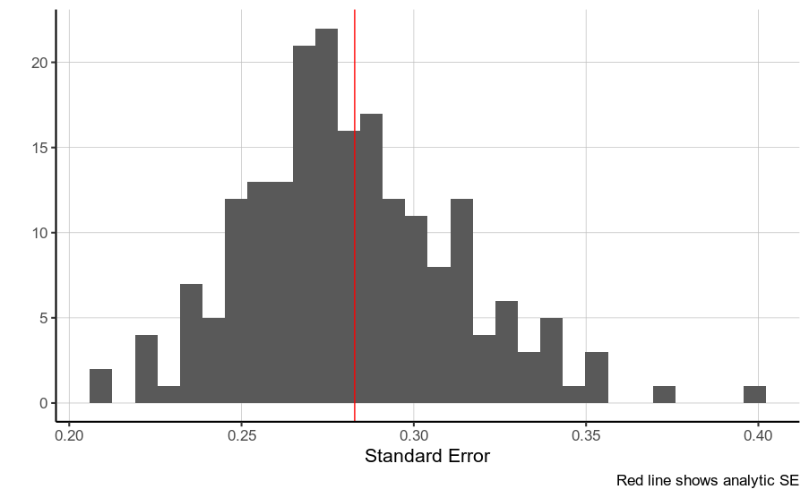
You can also test that the bootstrap estimate converges to the analytic solution:

sim_bootstrap = function(i){
  # Simulate fresh data
  X = rnorm(n, m, s)
  Y = rnorm(n, m, s)
  bootstrap_cov = map_dbl(1:nboot, function(i){
    # Do bootstrap sample
    rx = sample(X, n, replace = T)
    ry = sample(X, n, replace = T)
    cov(rx, ry)
  })
  sd(bootstrap_cov)
}
results = map_dbl(1:200, sim_bootstrap)
mean(results)
# [1] 0.2817101

qplot(results) + geom_vline(xintercept=expected_se, color='red') +
  labs(x='Standard Error', caption='Red line shows analytic SE')