Revisiting the Rule of Three

Question

The rule of three is a method for calculating a 95% confidence interval when estimating $p$ from a set of $n$ IID Bernoulli trials with no successes.

My understanding from its derivation is that the confidence interval it produces, $[0,\frac{3}{n}]$, is the interval which contains those values of $p$ such that,

$$\text{Pr}\big(\sum_{i=1}^n X_i=0\big)\geq0.05.$$

That is to say, those values of $p$ such that the chance of having no successes in $n$ trials is greater than or equal to 5%.

However in practice this approach does not produce confidence intervals which contain the true parameter 95% of the time.

For instance, suppose that $p=\frac{3}{n}+\varepsilon$. Then 5% of the time you will use the rule of three and your confidence interval will not contain $p$, and 95% of the time you will apply the standard CI prodecure using the sample standard deviation, and this confidence interval will contain $p$ approximately 95% of the time.

Hence we have the probability of your confidence interval containing $p$ given by,

$$0.05 \cdot 0 + 0.95^2 = 0.9025 \neq0.95.$$

Am I misunderstanding the rule of three? My analysis shows that it does not function as a rule for producing a 95% confidence interval.

Answer 1

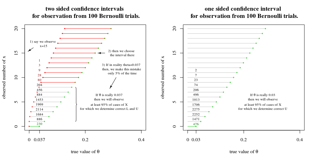
The image below is how I look at confidence intervals. It is an adaptation from an image in the answer to the question 'The basic logic of constructing a confidence interval', which is itself an adaptation of "The Use of Confidence or Fiducial Limits Illustrated in the Case of the Binomial C. J. Clopper and E. S. Pearson Biometrika Vol. 26, No. 4 (Dec., 1934), pp. 404-413"

For instance, suppose that $p=\frac{3}{n}+\varepsilon$. Then 5% of the time you will use the rule of three and your confidence interval will not contain $p$, and 95% of the time you will apply the standard CI prodecure using the sample standard deviation, and this confidence interval will contain $p$ approximately 95% of the time.

• One-sided boundaries

  The situation of the rule of three according to the derivation on Wikipedia is more close to the image on the right, which is for one-sided intervals. The boundary $3/n$ is the situation when you will observe less than 5% of the time zero successes. If the true value would be $3/n+\epsilon$ then you will make this error less than 5% of the time. In the other cases observations 1, 2, etc. You will always make the correct boundary if you consider one-sided boundaries. (you argue that in 95% of the cases you will be using the other interval and make 95% error in those cases, that is not true)

• Two-sided boundaries

  For the situation on the right the confidence interval for 0 observations is not $3/n$. For two sided intervals one computes the boundaries such you have in 5% probability (at most) to end up at both ends together. In the case of equal tails/sides then the boundary is computed such that $(1-p)^n \leq 0.025$, from which follows $$p \approx -\log(1-p) = -\log(0.025)/n \approx 3.7/n$$

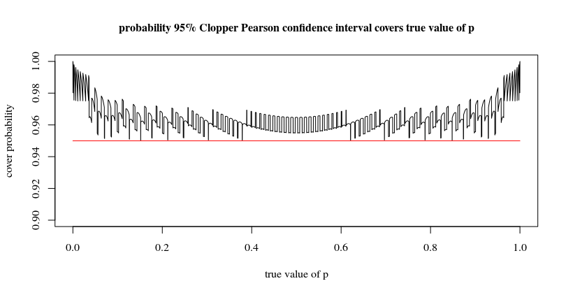
In the example above for $n = 100$ you see that the $3.7/n$ works well. You see also a problem with these boundaries in the case of binomial distributions. Due to the discreteness the method will not give exactly 95% probability for every value of $p$. Below is a plot for the coverage probability of the intervals as function of the parameter value

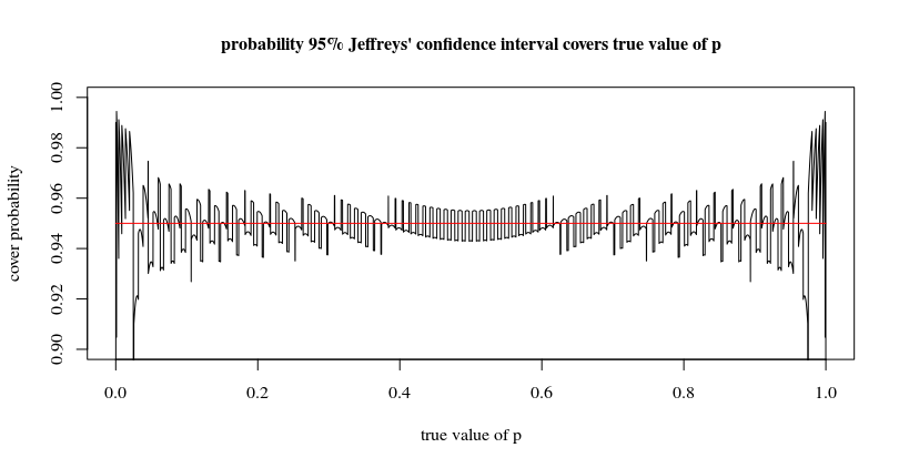
To be complete, we also plot Jeffreys' confidence interval, which BruceET mentions in his answer. It evens out the probabilities and makes the confidence interval smaller for $p$ close to $0$ and $1$. Conditional on the true value of the parameter, the Jeffreys' interval does not always cover the parameter with at least 95% probability, but it is also not designed to do that.

p_cover <- function(p, type = 1) {
  n = 100
  k = 0:n
  if (type == 1) { ### Clopper Pearson 
    p_upper = qbeta(1-0.025,k+1,n-k)
    p_lower = qbeta(0.025,k,n-k+1)
  } else { ### Jeffreys'
    p_upper = qbeta(1-0.025,k+0.5,n-k+0.5)
    p_lower = qbeta(0.025,k+0.5,n-k+0.5)
  }
  ks <- which((p <= p_upper)*(p >= p_lower)==1)
  sum(dbinom(ks-1,n,p))
}
p_cover <- Vectorize(p_cover)

ps <- seq(0,1,0.0001)

plot(ps,p_cover(ps), type = "l", ylim = c(0.9,1), 
    xlab = "true value of p",
    ylab = "cover probability",
    main = 
    "probability 95% Clopper Pearson confidence interval covers true value of p",
     cex.main = 1)
lines(c(0,1), c(0.95)*c(1,1), col = 2)

plot(ps,p_cover(ps, type = 2), type = "l", ylim = c(0.9,1), 
                xlab = "true value of p",
   ylab = "cover probability",
   main = 
   "probability 95% Jeffreys' confidence interval covers true value of p",
     cex.main = 1)
lines(c(0,1), c(0.95)*c(1,1), col = 2)

Answer 2

You can find some useful discussion of the "rule of three", including derivations and simulation analysis, in Javonovic and Levy (1997). With modern computing technology there is really no reason to use a "rule of thumb" like this instead of a good confidence interval formula what respects the support of the parameter of interest. For inference for a binomial proportion the Wilson score interval gives an interval that respects the support of the proportion parameter and has good large-sample properties. This interval reduces down to something similar (but not the same as) the "rule of three" when you have no successes. This aspect of the Wilson score interval is discussed in the paper O'Neill (2021) (p. 5), which sets out mathematical properties of the Wilson score interval, including the finite population correction for inference to a finite population or the unsampled part of a finite population.

---

Wilson score interval with no successes: Let $\chi_{1, \alpha}^2$ denote the critical point of the chi-squared distribution with one degree-of-freedom, using the upper-tail area $\alpha$. With no successes, the Wilson score interval is:

$$\text{CI}_p(1-\alpha) = \Bigg[ 0 , \frac{\chi_{1, \alpha}^2}{n + \chi_{1, \alpha}^2} \Bigg].$$

Taking $\alpha = 0.05$ for a 95% confidence interval gives:

$$\text{CI}_p(0.95) = \Bigg[ 0 , \frac{3.841459}{n + 3.841459} \Bigg].$$

For large $n$ this is fairly similar to the "rule of three" but it should be more accurate than this rule of thumb. As to showing that the rule has the required coverage probability, this holds using the normal approximation to the binomial for large $n$. One advantage of this interval over the "rule of three" is that it gives a valid value even for values $n=1,2$ where the "rule of three" goes outside the support of the parameter. (The Wilson score interval is not wonderful in these situations either, but at least it respects the support of the parameter!)

Answer 3

If you get no successes in (say) $n = 100$ trials, then you might use a Jeffreys Confidence interval for the true binomial $p.$ This style of CI has very good frequentist properties, but its motivation is in terms of a Bayesian argument using the non-informative prior distribution $\mathsf{Beta}(.5,.5).$ For $n = 100$ it gives the 95% CI shown in the R code below, which amounts to $(0.000, 0.025).$

qbeta(c(.025,.975), 0+.5, 100+.5)
[1] 4.898073e-06 2.474527e-02

If you want a one-sided CI (essentially 95% upper bound) then the the bound is 0.018.

qbeta(.95, 0+.5, 100+.5)
[1] 0.01897689

Notes: (1) I have never been a fan of the 'rule of three', even less nowadays when computation of more realistic intervals is so easy, using R. It seems that the rule of three is based on a kind of CI that has been shown not to have the claimed coverage probability.

(2) With no successes at all, there may be philosophical difficulties centering on whether the true success probability may be $0,$ so that no legitimate CI exists. In about 35 years of organized listening at various radio frequencies for messages from extraterrestrials, no such messages have been confirmed. Maybe there are no extraterrestrials with radio transmitters beamed in our direction.

Addendum re Comments: For given $n$, it is almost always possible to cherry-pick individual values of $p.$ for which any style of CI has poor coverage probability. If $n=100, p=0.021,$ then a "95%" Jeffreys CI has about 98% coverage probability, as computed in R below.

The discreteness of the binomial distribution implies swings in coverage probability for nearby values of $p.$ The idea is to pick a style of CI that does not get "too far" from 95% coverage for "most" of the values of $p$ of interest.

I am not claiming that Jeffries CIs are always best, only that I prefer them to the 'Rule of 3'. [The most relevant paper on such topics may be Brown, Cai & DasGupta (2001), Statistical Science.]

n = 100;  p = 0.021;  x = 0:100
lcl = qbeta(.025, x+.5, n-x+.5)
ucl = qbeta(.975, x+.5, n-x+.5)
cov = (p > lcl)&(p < ucl)
x.cov = x[cov]
sum(dbinom(x.cov,n,p))
[1] 0.9808197