3
$\begingroup$

I am new to Bayesian statistics. I am trying to understand a certain passage in my course notes.

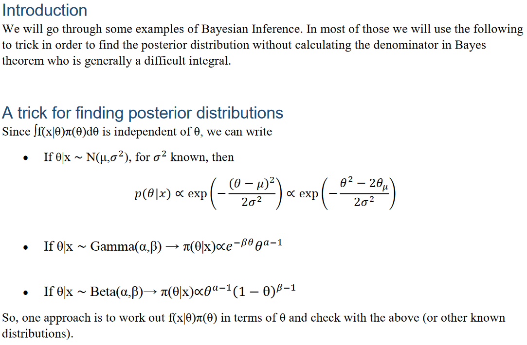
Excerpt:

enter image description here

Discussion:

I don't understand much about the above excerpt. I think that the goal here is to compute something along the lines of $\pi(\theta | x) = \frac{f(x | \theta) \pi(\theta)}{f(x)}$, where $f(x) = \int f(x | \theta) \pi(\theta)d\theta$. We are trying to turn our model for the data and the parameter into a posterior distribution for the parameter given the data.

I do not see what the trick is. What I see is that, for example, if $\theta | x \sim \text{Beta} (\alpha, \beta)$, then $\pi (\theta | x) = \frac{\theta^{\alpha - 1}(1 - \theta)^{\beta - 1}}{\text{B}(\alpha, \beta)}$, where the denominator is a constant (I think) so it follows that $\pi(\theta|x) \propto \theta^{\alpha - 1}(1 - \theta)^{\beta - 1}$.

I believe the same procedure works for the other two examples, in which you set up the equation for the known form of the density, strip out the constants, replace $=$ with $\propto$, and Bob's your uncle.

Or maybe the point is that if $\pi(\theta | x) = \frac{f(x | \theta) \pi(\theta)}{f(x)}$ where the denominator is a nasty integral, then it's simpler to write $\pi(\theta | x) \propto f(x | \theta) \pi(\theta)$. So maybe the upshot is that we perform the multiplication $f(x | \theta) \pi(\theta)$, see if it similar to a known distribution, and this gives us information about the type of distribution the posterior has.

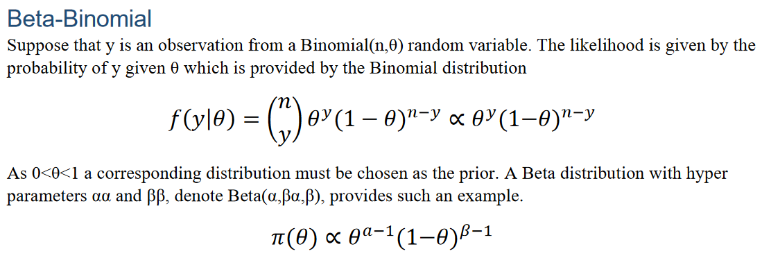
I think the subsequent example in the notes seems consistent with my expectations. (Sorry, these notes seem sloppily written.)

enter image description here enter image description here

I appreciate any help.

$\endgroup$
2
  • 2
    $\begingroup$ When prior and likelihood are 'conjugate' (mathematically compatible), one can notice the kernel (density without norming constant) of the posterior by looking at the product of prior and likelihood. In such cases, it is not necessary to evaluate the integral in the denominator of the posterior. // Your beta=binomial is a simple example of that. $\endgroup$
    – BruceET
    Commented Dec 7, 2020 at 21:40
  • 2
    $\begingroup$ @BruceET Thanks for the comment. That seems a lot simpler to understand than what my notes were trying to explain. $\endgroup$
    – Novice
    Commented Dec 7, 2020 at 21:45

1 Answer 1

4
$\begingroup$

This is a "trick" that applies more broadly than Bayesian statistics. It occurs whenever you know that a probability density function is proportionate to some known functional form. For example, suppose you have some non-negative function $g$ and you have a density function given by:

$$p(\theta|x) \propto g(\theta).$$

In this case, the norming axiom of probability means that there is only one possible solution for the density function --- it is the density that is proportionate to stipulated function and integrates to one:

$$p(\theta|x) = \frac{g(\theta)}{\int g(\theta) d\theta}.$$

Because there is a unique density function that is proportionate to any non-negative function $g$, this means that you can find densities just by "recognising" their proportionate forms (i.e., what they look like without their constant of integration). Here are a few of the continuous distributions:

$$\begin{matrix} \text{Normal density} & \text{N}(\theta|\mu, \sigma^2) \propto \exp \Big( -\frac{1}{2} (\frac{\theta - \mu}{\sigma})^2 \Big) & \text{ for } \theta \in \mathbb{R}, \\[6pt] \text{Student T density} & \quad \text{St}(\theta|\nu) \propto \Big( 1 + \frac{\theta^2}{\nu} \Big)^{-(\nu-1)/2} \ & \text{ for } \theta \in \mathbb{R}, \\[12pt] \text{Gamma density} & \text{Ga}(\theta|\alpha, \lambda) \propto \theta^{\alpha-1} \exp (- \theta/\lambda) \quad & \text{ for } \theta \geqslant 0, \\[16pt] \text{Weibull density} & \quad \text{Wei}(\theta|\alpha, \beta) \propto \theta^{k-1} \exp (- (\theta/\lambda)^k) \quad \ \ & \text{ for } \theta \geqslant 0, \\[16pt] \text{Beta density} & \quad \text{Be}(\theta|\alpha, \beta) \propto \theta^{\alpha-1} (1-\theta)^{\beta-1} \quad \quad \ & \quad \ \ \ \text{ for } 0 \leqslant \theta \leqslant 1. \\[12pt] \end{matrix}$$

In the context of Bayesian statistics, it is common to use proportionality to simplify the derivation of posterior densities, using the kind of working shown in your question. In this context we generally ignore constant multiplicative terms and just find what function the posterior is proportionate to. We then either "recognise" this as a standard distributional form, or if it is not a standard form we determine the constant of proportionality by integrating the function over its full range. (Sometimes there is no closed-form expression for the constant of integration, in which case we use numerical methods to estimate this constant, or we generate values from the posterior using MCMC methods.) By ignoring multiplicative constants in our working, and then bringing them back in in the last step, we greatly simplify Bayesian analysis.

Note that the above result is a general probability rule that applies more broadly than Bayesian statistics, but it is particularly helpful in this context because of the standard result that the posterior is proportionate to the product of the likelihood and prior.

$\endgroup$
0

Your Answer

By clicking “Post Your Answer”, you agree to our terms of service and acknowledge you have read our privacy policy.

Not the answer you're looking for? Browse other questions tagged or ask your own question.