how does the posterior predictive distribution account for differences in uncertainty?

Question

Recent research in the field of bayesian deep learning allows for the quantification of uncertainty in estimates of ML models. This can be done because the posterior predictive distribution of the model can be computed. Bayesian methods allow us to be more uncertain over regions where the model has not seen data. The example below illustrates this point. Picture is taken from A bayes by backprop implementation of a neural network

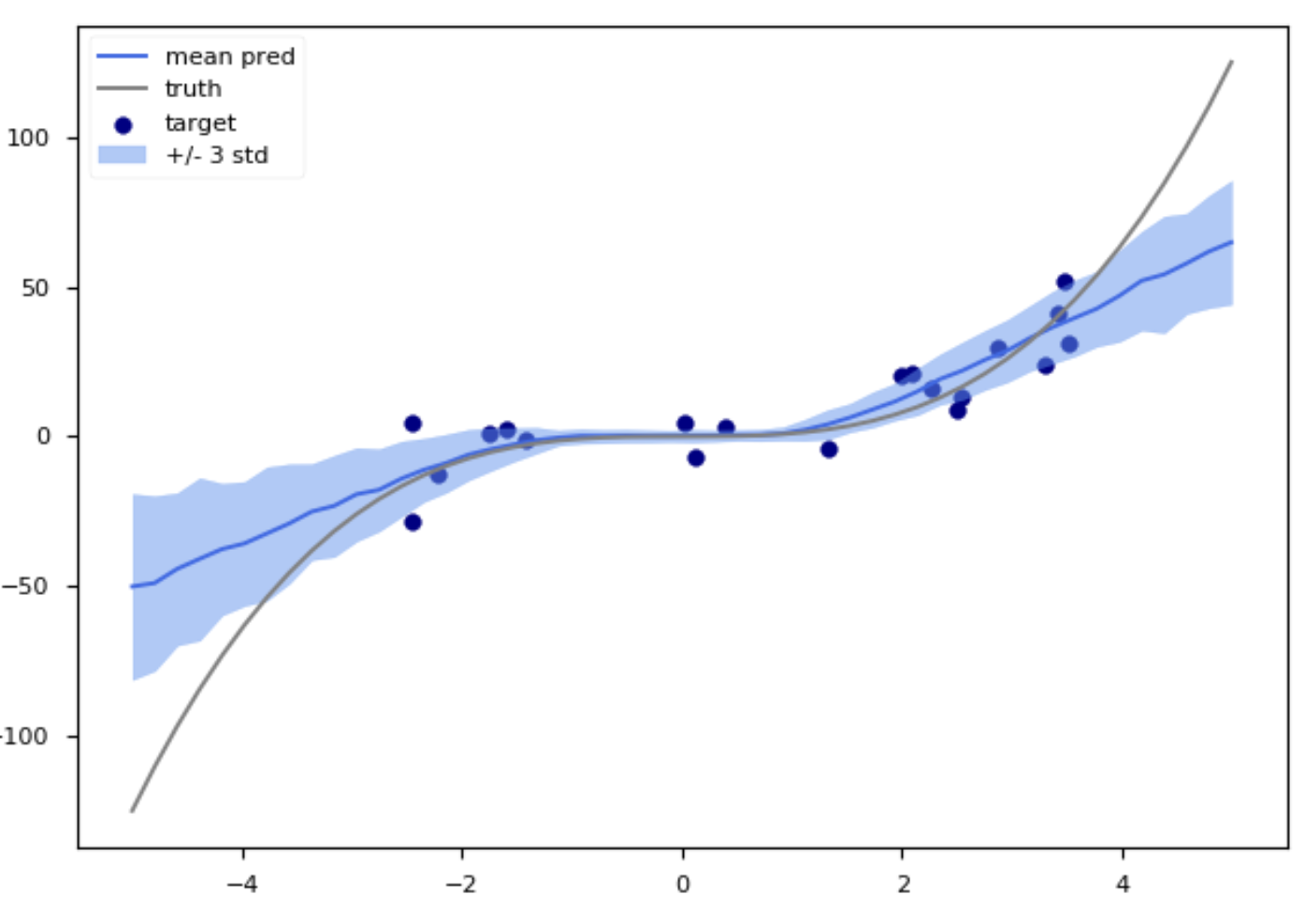
The distribution for $y^*$ given each $x^*$ (denoted by the coloured regions) is obtained by averaging the distribution $p(y^*|x^*,\theta)$ over empirical $\theta$ values sampled from the posterior over model weights. The posterior predictive distribution is computed as $$p(y^*|x^*) = \int p(y^*|x^*,\theta)p(\theta|X)d\theta$$

My question is how does the equation for posterior predictive result in a wider distribution for samples in which the model has not "seen"(Eg. $x$ values that are $>$ 4 and values that are $<$ -4) as compared to samples that are within the range of $-2 < x < 2$ ?

The current intuition I have on why uncertainty estimates are larger at regions in which the model has not seen the data is because the posterior weight distributions will lie in a region that can try to best explain how data "fed into" the model was generated. The likelihood for samples which are not seen by the model is very low under the posterior weights. When the posterior weights are sampled and the distribution of $y^*$ plotted under the different weights, I do not know why the variance is large for these "unseen" data.

Hope my question is clear.

Answer 1

For me, I think a helpful way to reason about this is to step back and think about polynomials. I'll make a little example with a cubic polynomial, since the truth in your picture appears to be cubic.

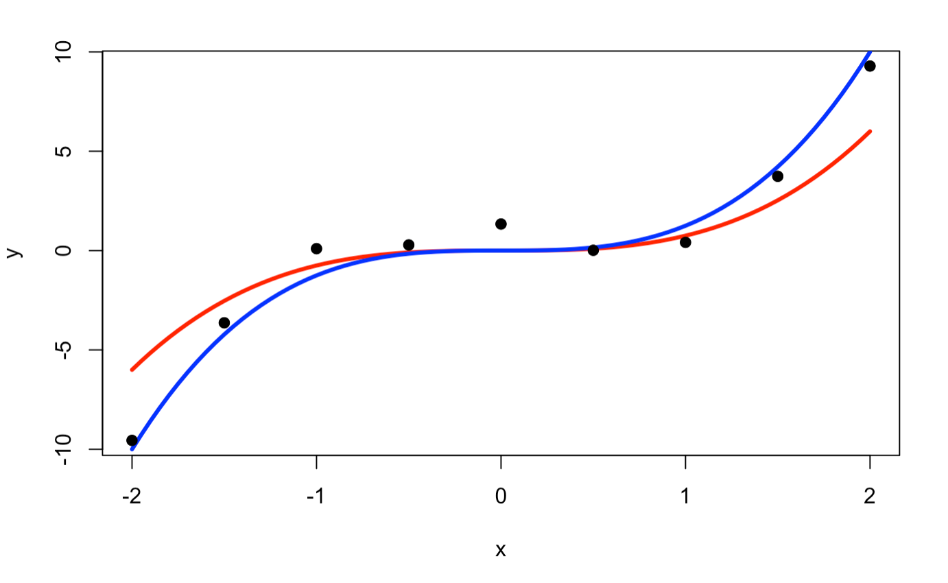
Let the true data-generating process be $$ y=\theta x^3, \text{ where } \theta=1. $$ I'll add some $N(0,1)$ noise and plot this in the picture below for some $x$ values in $[-2,2]$.

Now let's pretend I fit my Bayesian model and compute $p(\theta|y)$. Let's say I draw twice from this distribution and get $\theta^{(1)}=.75$ and $\theta^{(2)}=1.25$. To experiment, let's see what the cubic curves look like with these coefficients. Below they're plotted in red and blue.

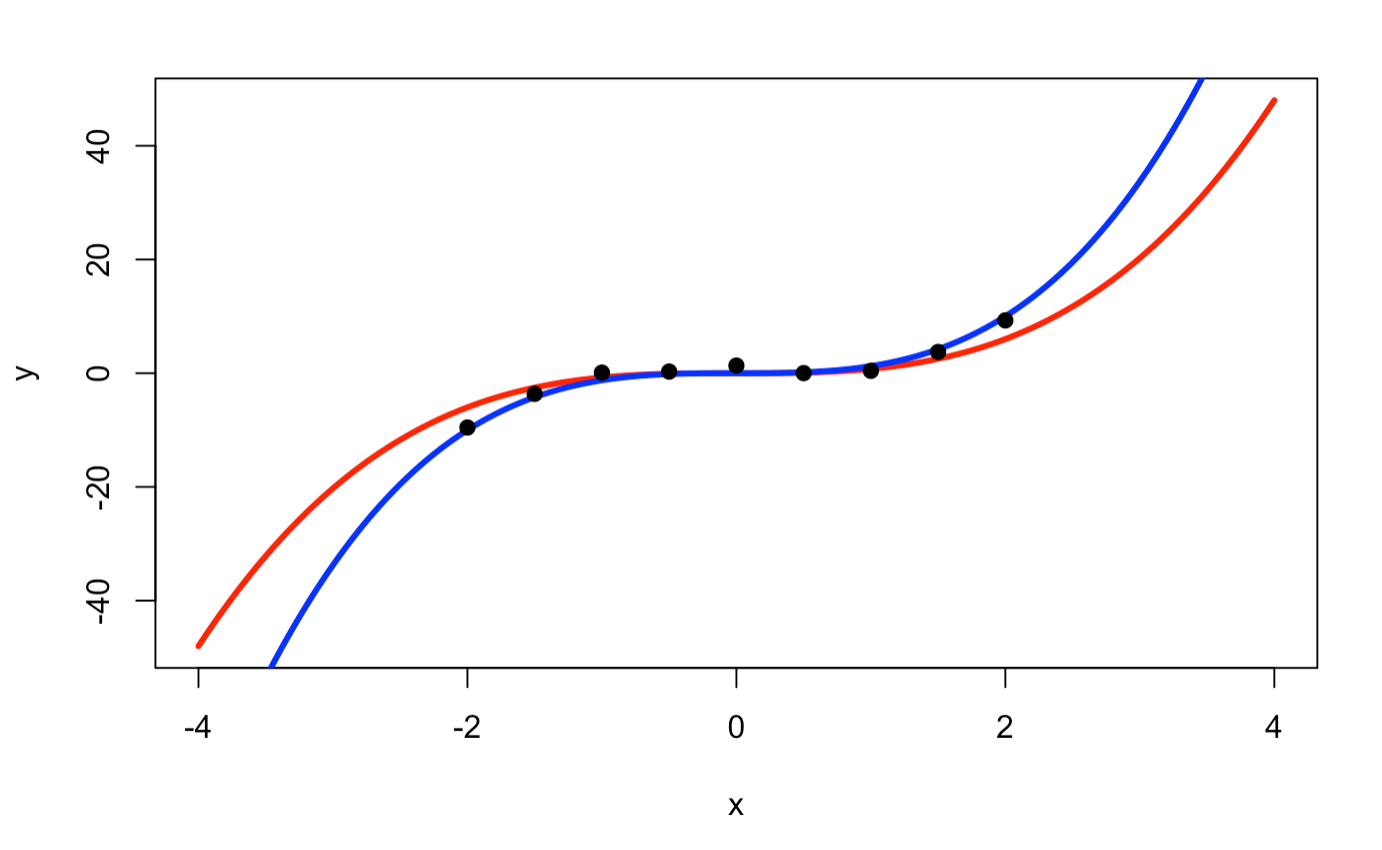
If you squint and close one eye, both fit the data decently. But what if I zoom out to $[-4,4]?$ Here you can see the curves are really starting to behave differently, and this gets at the heart of why you can think about the tails getting wider for your scenario. Since we haven't observed data at points $<-2$ or $>2$, the model doesn't "know" which parameter values are best.

Additionally, the posterior predictive distribution in practice is computed by first sampling (using your notation) $\tilde\theta\sim p(\theta|X)$ and then sampling $p(y^*|x^*,\tilde\theta)$. So if we repeat this process many many times, we're going to get wider intervals for the posterior predictive distribution just because lots of different $\theta$ values have been sampled. The cubic curve is very sensitive to the $\theta$ draws as we move away from the origin. But near the origin, many values of $\theta$ are roughly compatible with the observed data.

That was all informal and heuristic, but hopefully it helps. cheers