Is the median of expected values equal to the expected value of median?

Question

Suppose that an individual $i$ earns $X_{1_i}$ with probability $P_i$ and $X_{2_i}$ with probability $1-P_i$. The expected value of income can be expressed as $E(X_i)=P_i\cdot X_{1_i}+(1-P_i)\cdot X_{2_i}$. Suppose there are $N$ individuals with unique values of $P$, $X_1$, and $X_2$, such that $P_i\neq P_j$, $X_{1_i}\neq X_{1_j}$, and $X_{2_i} \neq X_{2_j}$. It is straightforward to compute the median of $E(X)$.

Suppose I construct a simulation of the situation described above where for each individual $i$ I draw once from the following Bernoulli distribution:

$$E_i \sim B[P_i]$$

and then assign income as follows:

\begin{equation} X_i= \left\{ \begin{array}{ll} X_{1_i} & \text{if}\space E_i=1 \\ X_{2_i} & \text{if}\space E_i=0 \end{array} \right. \end{equation}

I can then compute the mean of $X$. If I run this simulation $k$ times I obtain $k$ median values. Should I expect the average of these $k$ observations of the median to converge to the median of $E(X)$? Is there some theorem that proves this? Or am I missing the forest for the trees somehow with my logic. Thanks!

Answer 1

Your example. Suppose $P(X = 20) = 0.6$ and $P(X = 40) = 0.4.$ Then $\mu= E(X) = 20(.6)+40(.4) = 12+16 = 28.$ Also, $\eta = Med(X) = 20$ because $P(X < 20) = 0 < 0.5$ and $P(X > 20) = 0.4 < 0.5.$

Now we use R to sample $n=100\,000$ observations $X_1, X_2, \dots, X_n$ from this distribution.

set.seed(2020)
x = sample(c(20,40), 10^5, rep=T, p=c(.6,.4))

A tabulation of results shows that we have about 60% 20s and about 40% 40s.

table(x)/10^6
x
     20      40 
0.60473 0.39527 

A summary of sample statistics shows that the median of this large sample $H = 20.0$ is the same as the median $\eta=20$ of the distribution; and the mean $A = \bar X = 27.91$ is very nearly the same as the mean $\mu = 28$ of the population.

summary(x);  var(x)
   Min. 1st Qu.  Median    Mean 3rd Qu.    Max. 
  20.00   20.00   20.00   27.91   40.00   40.00 
[1] 95.61361   # sample variance S^2

The general principle is that for increasingly large samples, the sample mean converges to the population mean and the sample median converges to the population variance.

Furthermore, the population variance is $$\sigma^2= Var(X_i) = P(X=20)(20-\mu)^2 + P(X=40)(40-mu)^2 \\ = 0.6(20-28)^2 + 0.5(40-28)^2 = 96.$$ And the sample variance $S^2 =95.61$ has nearly the same numerical value.

Binomial Example. This same kind of convergence holds true for more complicated distributions. For example, The number $Y$ of heads in ten tosses of a fair coin has the distribution $\mathsf{Binom}(n=10, p=1/2).$ This distribution has $\mu_Y = E(Y) = np =10(1/2) = 5,$ median $\eta_Y = 1/2,$ and variance $\sigma^2_Y = Var(Y) = np(1-p) = 5/2 = 2.5.$

Suppose we use R to sample $m = 100\,000$ results $Y_i.$

set.seed(1224)
y = rbinom(10^5, 10, .5)
summary(y);  var(y)
   Min. 1st Qu.  Median    Mean 3rd Qu.    Max. 
  0.000   4.000   5.000   4.988   6.000  10.000 
[1] 2.483412

The sample mean $\bar Y = 4.988 \approx \mu_Y = 5,$ Also, the sample median $5.000$ matches the population median $\eta = 5,$ and the sample variance $S_Y^2 = 2.4835 \approx \sigma_Y^2 = 2.5.$

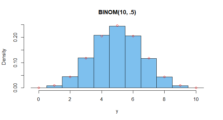
Moreover, if we make a histogram of the $m = 100\,000$ simulated values of $Y$ (blue), the heights of the histogram bars nearly match the probabilities that $Y$ takes the corresponding values (red circles).

hist(y, prob=T, br=-.5:10.5, col="skyblue2", main="BINOM(10, .5)")
 k = 0:10;  pdf = dbinom(k, 10, .5)
 points(k, pdf, col="red")