Not rejecting null-hypothesis and inflation of type I error

Question

Context

In statistics, it is quite common to perform statistical tests in the explicit goal of not-rejecting the null hypothesis. For example, prior to conducting an ANOVA, one will check for homogeneity of variances (F-test, Bartlett Test).

I have the feeling that doing so is quite dishonest since each of these tests always have unknown type II error and this is similar to saying : "My assumption is that I am a unicorn, prove me wrong" while the burden of proof should be on claiming that "variances are similar" and not the other way around.

Problem

If one wants to test that Group A is different than Group B and Group C and thus follows this general routine :

1. Test for homogeneity of variances and do not reject H0 (type II error unknown)
2. ANOVA test is statistically significant ( .05 level)

Considering that unknown type II error, can we really say that the Type I error is only 5 % ?

Answer 1

1. A test can never make sure that the model is correct. What tests do is that they check the compatibility of the data with the model, i.e., could the model realistically have produced such data? You are right that a non-rejection does not prove the model - regardless of what the "explicit goal" was.

2. You are also right that technically one can therefore object to a procedure that implies that a certain model assumption is fulfilled just because a test of the model did not reject the model assumption.

3. The statement that "the Type I error is only 5%" refers to what I call the "model-world", not the real world. It says that if the model is correct, the rejection probability is 5%. This is a technically correct statement regardless of what the practical situation is. It however does not give you a guarantee in practice; you should not believe something like that you'd now be 95% sure that the model holds.

4. Given that models never hold precisely in reality, the aim of a misspecification test (like testing homogeneity of variances) is not quite what people normally say it is. Actually this is done not because it could make sure that the model holds with large probability (it can't, as explained above). Rather it is done to indicate that a potential violation of the assumption is not strong and strikingly clear. True, the test cannot confirm the model, but it can make sure that the data are not obviously far away from it. The hope is that, although the model may be violated in a certain way, it is not violated in such a way to invalidate the conclusions you draw from it. The aim is, rather more modestly than making sure that the model assumptions hold, to do something with the data that is not obviously contradicted by them.

5. Whether this is a good approach is controversial and unfortunately depends on all kinds of details (what exact misspecification test you run, what is your alternative action in case the misspecification test rejects the assumption, how exactly is the assumption violated that you are testing). There is some literature that investigates testing homogeneity of variances and then conditionally on it to run a standard two-sample test or ANOVA, and the results are not very encouraging for this kind of "combined procedure" - in the specific setup treated by BruceET's answer I'd agree with the advice given there -, although it does help in some other situations. See this arxiv paper for a recent literature overview and discussion:

   https://arxiv.org/abs/1908.02218

6. Unfortunately the problem does not go away by not running formal misspecification tests and instead looking at the data and deciding whether an assumption looks OK. The problems with this are the same in principle, but because of the subjective nature they cannot be formally analysed, so there is no literature quantifying problems with this approach. This doesn't mean that they don't exist. Visual checking certainly has its role to play, but I have met people who think that formal misspecification tests should not be used because of the problems that you have alluded to and that are elaborated in the paper linked above and the literature cited there, however looking at graphs and deciding what to do based on them is fine. Not so - there is really no escape. We have to live with the fact that we are working with model assumptions that ultimately we have no way to verify.

Answer 2

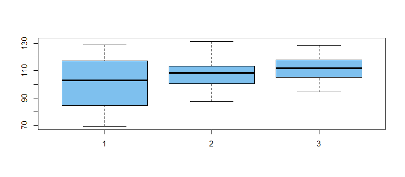
If you doubt that groups A, B, C are from populations with equal population variances, but believe that data are reasonably close to normal, then you can use a version of a one-way ANOVA that does not require equal variances. In R, this procedure is oneway.test. [This would be analogous to choosing a Welch two-sample t test instead of a pooled t test, if you had only two levels of the factor.]

Here is an example:

set.seed(2021)
a = rnorm(32, 101, 16)
b = rnorm(30, 110, 10)
c = rnorm(40, 114, 9)
x = c(a,b,c)
g = as.factor(rep(1:3, c(32,30,40)))
boxplot(x~g, col="skyblue2")

oneway.test(x ~ g)

     One-way analysis of means 
   (not assuming equal variances)

data:  x and g
F = 4.6551, num df = 2.000, denom df = 55.596,
p-value = 0.01351

Not assuming equal variances, oneway.test finds a significant difference at the 2% level. [An ad hoc Welch 2-sample t test finds a significant difference between a and c, but not for the other comparisons among levels.]

t.test(a,c)$p.val  # Welch 2-sample t test
[1] 0.007086897

By contrast, a standard ANOVA (incorrectly assuming equal variances) finds a significant difference at the lower 1% level, which is not justifiable in view of the unequal variances among levels. [Notice that oneway,test uses denominator DF = 55, as a 'penalty' for unequal variances, while the standard ANOVA uses DDF = 99.]

anova(lm(x~g))
Analysis of Variance Table

Response: x
          Df  Sum Sq Mean Sq F value   Pr(>F)   
g          2  1757.8  878.88  5.3814 0.006045 **
Residuals 99 16168.5  163.32                    
---
Signif. codes:
0 ‘***’ 0.001 ‘**’ 0.01 ‘*’ 0.05 ‘.’ 0.1 ‘ ’ 1

Unless you are quite sure--based on previous knowledge or experience with similar data--that levels of such a factor must have nearly equal variances, it is good practice to do the version of the ANOVA that does not assume equal variances. Tests for equal variance are known to have low power, so 'branching' to one kind of ANOVA or the other based on such a test is not a good idea. If there is a question about the normality of the data, it may be best to use a nonparametric "ANOVA" (possibly a permutation test).

---

Note: Example of a permutation test.

The major finding from my (fake) data above was that sample means for A and C are statistically different.

Regardless of its distribution, suppose I am willing to use the Welch t statistic as a reasonable measure ('metric') of the distance between $\bar X_A$ and $\bar X_C.$ Under the null hypothesis $H_0:\mu_A = \mu_B,$ it should not matter which of the $32+40 = 72$ observations comes from which group.

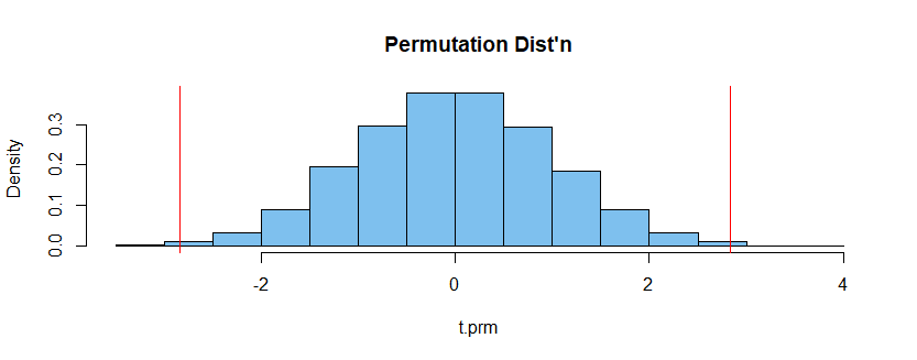
By repeatedly re-assigning the observations at random to groups of sizes $32$ and $40$ and computing the Welch t statistic for each assignment, I can get a good idea of the permutation distribution of that statistic. This method of approximating the permutation distribution does not depend on the normality or homoscedasticity of the data.

Then, if the observed Welch t from the actual assignment is sufficiently far into a tail of the permutation distribution, I can reject $H_0.$

AC = c(a,c);  G=rep(1:2, c(32,40))
t.obs = t.test(AC~G)$stat
set.seed(101)
t.perm = replicate(10^5, t.test(AC~sample(G))$stat)
mean(abs(t.perm) >= abs(t.obs))
[1] 0.00617   # P-value of permutation test
hist(t.prm, prob=T, col="skyblue2", main="Permutation Dist'n")
 abline(v=c(-t.obs, t.obs), col="red")