2
$\begingroup$

I've been reading this blog post, which has been tremendously helpful in understanding Gaussian Processes (GP.) The author has used the terms "prior", "posterior", and "95% confidence interval" throughout; this made it difficult for me to tell if he was approaching GP from a Frequentist or Bayesian perspective. In equation 11, he defines the log marginal likelihood then uses scipy to optimize the hyperparameters, L and Sigma. He doesn't explicitly call it "MLE" but the concept seems analogous enough for me to consider his approach Frequentist. (Is this valid?)

And if so, how might a Bayesian approach GP? My currently thinking is: Rather than optimize the log marginal likelihood for point estimates of L and Sigma, sample hyperparameter values from the joint distribution. (Is this valid?)

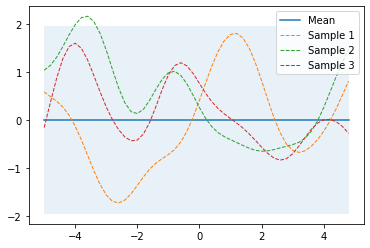
Lastly, the author makes some decisions that made the distinction between paradigms a little blurry for me. Namely, early in the article he discusses the prior, sets arbitrary values for L and Sigma, generates some fake X input data, then uses the Kernel(X,X) to generate a multivariate gaussian (w/ one dimension per data point) and samples from this multivariate gaussian 3 times to show what this "prior over functions might look like". And this has caused me a decent amount of confusion as it sounds quite Bayesian.

GP Prior

Could anyone offer some clarification?

Edit: Wow, there is no agreement on this topic, see extended conversation.

$\endgroup$
4
  • $\begingroup$ I think some of the redditors in your linked post are overthinking this.. How could a frequentist approach to GP regression here even make sense when there aren't even data for the majority of $x_i$? Like in that blog here there are only 5 data points constraining the joint distribution of 50 random variables $f(x)$ for $x \in$arange(-5,5,0.2). The resulting "fit" is evidently just the prior you pictured above updated in a Bayesian manner with the 5 data points. $\endgroup$
    – jnez71
    Commented Jan 4, 2021 at 18:58
  • $\begingroup$ @jnez71, as an aside, I'm starting to view GP regression as a weighted avg of a potentially inf sequence, where a given input, $x_i$ is pulled most strongly by itself and to lesser degrees by any other $x_j$ proportional to their distance away. So the kernel is just a means to evaluate how much a given $x_i$ should be weighted by all possible $x_j$. The regression happens when these weights are applied to the corresponding $y_j$ vector. This clears up why a mean vector is often 0. And makes intuitive why train data cannot be discarded at inference, as weights must still be learned. $\endgroup$
    – jbuddy_13
    Commented Jan 4, 2021 at 19:23
  • 1
    $\begingroup$ "x_i is pulled most strongly by itself and to lesser degrees by any other x_j" That would only be the case for a prior kernel like the radial basis kernel (very common choice, but not required). I think I agree with the rest of your intuition though. The real issue with GP is that we really need to work with a covariance function (not finite-dimensional matrix) and if we could update our prior covariance function (e.g. $K(t,t')=\sigma e^{-\frac{||t-t'||^2}{2l^2}}$) analytically then we would be able to discard the training data. $\endgroup$
    – jnez71
    Commented Jan 4, 2021 at 20:07
  • $\begingroup$ Instead, we suffice for a discretization that has to be "re-aligned" to the test points we want to infer. The re-alignment involves recomputing the Bayesian update, so we have to keep the training data around. Btw this Distill article does a much better job explaining GP than the linked blog imo. $\endgroup$
    – jnez71
    Commented Jan 4, 2021 at 20:10

1 Answer 1

3
$\begingroup$

Gaussian-process (GP) regression is almost always handled in a Bayesian manner. When people talk about "picking the right kernel" for their GP, they mean for the prior, and it has a dramatic effect on the predictions they make once updated via data to their posterior. The article you linked makes this idea pretty clear.

The author's use of the term "confidence interval" is a misnomer. They are just plotting the spread as dictated directly by the covariance matrix of the assumed Gaussian distribution. These are actual probabilities over the thing being estimated. I.e. your picture of the author's prior could be described as "$f(x_i)$ under the prior has a 95% probability of being between -2 and 2 $\forall i$."

The "marginal likelihood" maximization in Eq.11 is not the "training" (the "training" is the Bayesian updating of the prior GP to the posterior GP). Rather, it is sort of data-driven tuning of the prior by selecting kernel hyperparameters that maximize the "evidence" (denominator in Bayes rule), which the author calls "marginal likelihood."

$\endgroup$
2
  • $\begingroup$ Okay. So the author’s use of optimization is more akin to MAP than MLE (given that GP is almost exclusively a Bayesian construct, as you’ve noted.) In contrast, PyMC3 uses HMC/NUTS to sample distributions around kernel hyper parameters. But fundamentally, both MAP and MCMC fall under the realm of Bayesian statistics. So it’s not correct to label the author’s approach as frequentist. Is this a fair summary? $\endgroup$
    – jbuddy_13
    Commented Jan 4, 2021 at 17:25
  • 1
    $\begingroup$ @jbuddy_13 : I think so. I definitely agree with "it's not correct to label the author's approach as frequentist." $\endgroup$
    – jnez71
    Commented Jan 4, 2021 at 17:30

Your Answer

By clicking “Post Your Answer”, you agree to our terms of service and acknowledge you have read our privacy policy.

Not the answer you're looking for? Browse other questions tagged or ask your own question.