Adjusting P values for multiple comparisons using permutation tests

Question

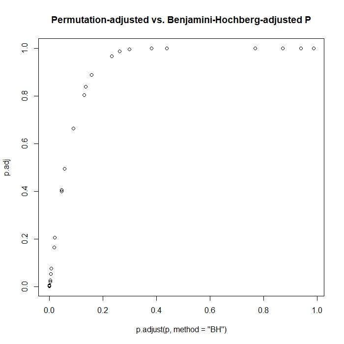
I have a number of continuous predictors (biomarker measurements) which I would like to test for association with a binary outcome variable (disease status), adjusting for multiple comparisons. As some of my predictors are correlated, I understand that procedures such as Benjamini-Hochberg might not be valid, so I would like to use permutation testing to adjust for multiple comparisons.

I did not manage to find an R code to do it, so I wrote it myself and used example data (see below). I wonder:

1. whether the code is correct for calculating P values adjusted for multiple comparisons using permutation testing?
2. if I did something wrong, as contrary to what I expected, P values adjusted for multiple comparisons using permutation testing are higher than e.g. Benjamini-Hochberg-adjusted P values?
3. why P values adjusted for multiple comparisons using permutation testing do not always increase monotonically with (unadjusted) permuted P values?

Here is the code:

Prepare example data:

library(mlbench)

data(Ionosphere)

Ionosphere <- Ionosphere[-c(1:2)]  # Remove factor variables.

dim(Ionosphere)
# [1] 351  33

# Columns 1-32: continuous independent variables.
# Column 33: binary dependent variable ('Class': bad/good).

Calculate original and permuted P values:

# Calculate original P values:

p <- sapply(
  Ionosphere[-ncol(Ionosphere)],
  function(x) {
    wilcox.test(x ~ Ionosphere$Class)$p.value
  }
)

# Permute:

n.perm <- 999

perm.matr <- rbind(
  p,  # Original P values included as one of the permutations.
  matrix(, nrow = n.perm, ncol = length(p))
)

set.seed(123)

system.time(

  for (i in 1:n.perm) {
  
    temp <- Ionosphere
  
    temp$Class <- sample(temp$Class)
  
    perm.matr[i + 1, ] <- sapply(
      temp[-ncol(temp)],
      function(x) {
        wilcox.test(x ~ temp$Class)$p.value
      }
    )
  
    rm(temp)
  
  }
  
)
  #  user  system elapsed 
  # 76.14    0.06   76.35 

rm(i)

# Calculate permuted P values:

p.perm <- apply(
  perm.matr,
  2,
  function(x) {
    sum(x <= x[1]) / length(x)  # x[1] is the original P value
  }
)

Calculate P values adjusted for multiple comparisons using permutation testing:

Based on this link.

p.adj <- as.numeric(rep(NA, length(p)))

names(p.adj) <- names(p)

for (i in 1:length(p)) {
  
  p.adj[i] <- sum(
    apply(
      perm.matr,
      1,
      min
    ) <= p[i]
  ) / nrow(perm.matr)
  
}

rm(i)

plot(
  p.adj ~ p.adjust(p, method = "BH"),
  main = "Permutation-adjusted vs. Benjamini-Hochberg-adjusted P"
)

An example where permutation-adjusted P values increase, but (unadjusted) permuted P values decrease:

This happens also with a higher number of permutations, e.g. n.perm = 9999.

This example also shows the discrepancy between the permutation-adjusted P values and Benjamini-Hochberg-adjusted P values.

data.frame(
  P = round(p, 4),
  P.permuted = p.perm,
  P.adjusted.perm = p.adj,
  P.adjusted.BH = round(p.adjust(p, method = "BH"), 4)
)[order(p), ][11:12, ]
#          P P.permuted P.adjusted.perm P.adjusted.BH
# V21 0.0031      0.006           0.075        0.0085
# V4  0.0032      0.003           0.076        0.0085

Answer 1

I can't answer your three numbered questions, but it seems to me that 'correction' of the p-values is not of any scientific utility in this setting. This can only be a preliminary study if you have so many biomarkers in play, so do not discard potentially useful markers because of the power-robbing effect of multiple comparison adjustments.

The p-values that you have are indices of the strength of evidence in the data against each null hypothesis relating to each predictor. If you perform a 'correction' for multiplicity then you are discounting those indices of evidence in favour of protection against increased false positive errors relative to a meta hypothesis that is unlikely to be of interest to you. That meta hypothesis is the global hypothesis that none of the individual null hypotheses are true.

You already know more about the biomarkers than the statistical model can, so your reaction to the p-values is more insightful than the statistical model's. Look at the p-values while considering the particulars of the biomarkers and decide which ones are worth following up upon (i.e. which are 'significant' in Fisher's sense). The second study will identify any false positive leads from the preliminary study without the cost of possibly discarding more truly useful markers.

Answer 2

Not a full answer - p values 0.0031 and 0.0032 are very close. Even with 10,000 permutations you are looking at the difference between 31 vs 32 samples passing the observed cutoff. So it may be just by chance that you see an inconsistency between your method and Benjamini-Hochberg's?