Estimating ability with IRT when item parameters are known using R package mirt

Question

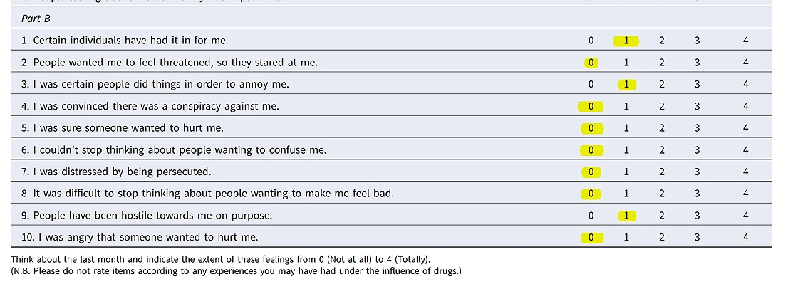
I have a paper which has utilised IRT on a revised scale of paranoia (R-GPTS). The scale comprises 10 items and there are 5 response options:

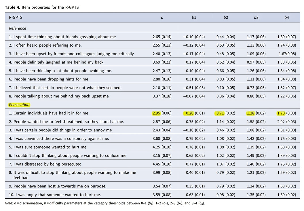
In the above highlighted responses, this scores 3 / 40. The item parameters are for the persecution subscale:

I am trying to get an ability estimate but I can tell that I'm missing something.

This is the IRT model the authors used:

A two-parameter graded response model (GRM) was fitted to the items (Samejima, 1969).

These are the packages they used:

All analyses were conducted in R, version 3.5 (R Core Team, 2013). Packages used included ‘psych’ >(Revelle, 2018), ‘mirt’ (Chalmers, 2012), ‘pROC’ (Robin et al., 2011), and ‘optimumCutpoints’ (Lopez-Raton et al., 2014).

In Estimating ability using IRT when the model parameters are known there is a response by philchalmers who wrote mirt, the very package used in the study. Taking his code I have come up with the following:

#generates set of random response patterns for 10 items
dat <- matrix(sample(c(0,1,2,3,4), 20000, TRUE), ncol=10)
colnames(dat)<-paste0('Item', 1:10)

library(mirt)

#2PL polytomous or graded response model from Samejima 1969
sv<-mirt(dat, 1, itemtype= 'graded', pars = 'values')


#item parameters from Freeman et al. 2019
sv$value[sv$name == 'a'] <- c(2.95,2.87,2.43,3.68,4.25,3.15,4.45,3.99,3.54,3.59)
sv$value[sv$name == 'b1'] <- c(0.20,0.75,−0.10,0.79,0.78,0.65,0.77,0.40,0.35,0.63)
sv$value[sv$name == 'b2'] <- c(0.71,1.14,0.46,1.08,1.08,1.02,1.07,0.79,0.79,0.98)
sv$value[sv$name == 'b3'] <- c(1.28,1.58,1.08,1.43,1.39,1.49,1.40,1.21,1.24,1.35)
sv$value[sv$name == 'b4'] <- c(1.70,2.02,1.61,1.75,1.68,1.89,1.75,1.59,1.63,1.69)

#set item parameters as fixed
sv$est<-FALSE

mod<-mirt(dat, 1, pars=sv)

Then, I use fscores() for ability estimate:

# response pattern #1
fscores(mod,response.pattern=c(1,0,1,0,0,0,0,0,1,0))

# response #2
fscores(mod,response.pattern=c(4,0,4,4,3,3,4,4,4,4))

# response #3
fscores(mod,response.pattern=c(4,0,4,4,4,4,4,4,4,4))

The output I get is as follows:

> # response pattern #1
> fscores(mod,response.pattern=c(1,0,1,0,0,0,0,0,1,0))
     Item1 Item2 Item3 Item4 Item5 Item6 Item7 Item8 Item9 Item10        F1     SE_F1
[1,]     1     0     1     0     0     0     0     0     1      0 -2.078653 0.5700438
> 
> # response #2
> fscores(mod,response.pattern=c(4,0,4,4,3,3,4,4,4,4))
     Item1 Item2 Item3 Item4 Item5 Item6 Item7 Item8 Item9 Item10       F1     SE_F1
[1,]     4     0     4     4     3     3     4     4     4      4 1.856076 0.5946364
> 
> # response #3
> fscores(mod,response.pattern=c(4,0,4,4,4,4,4,4,4,4))
     Item1 Item2 Item3 Item4 Item5 Item6 Item7 Item8 Item9 Item10       F1   SE_F1
[1,]     4     0     4     4     4     4     4     4     4      4 2.352869 0.63262

Now, although the #2 and #3 look about right, the whole problem is that I really don't think #1 should have $\theta$ = -2.0. In their study the authors report a mean score of about 2.3 I should be getting closer to $\theta$ = 0.

However, the strangest thing is that in abovementioned post there is a suggestion to use catR. Using this package I'm getting ability estimates that I think are correct.

Here is my code:

library(catR)

pars<-data.frame(a=c(2.95,2.87,2.43,3.68,4.25,3.15,4.45,3.99,3.54,3.59),
b1=c(0.20,0.75,−0.10,0.79,0.78,0.65,0.77,0.40,0.35,0.63),
b2=c(0.71,1.14,0.46,1.08,1.08,1.02,1.07,0.79,0.79,0.98),
b3=c(1.28,1.58,1.08,1.43,1.39,1.49,1.40,1.21,1.24,1.35),
b4=c(1.70,2.02,1.61,1.75,1.68,1.89,1.75,1.59,1.63,1.69))

#item  parameters from Freeman et al. 2019
pars

#estimate for response pattern #1
thetaEst(pars, c(1,0,1,0,0,0,0,0,1,0), model = "GRM", method = "EAP")

#estimate for response pattern #2
thetaEst(pars, c(4,0,4,4,3,3,4,4,4,4), model = "GRM", method = "EAP")

#estimate for response pattern #3
thetaEst(pars, c(4,0,4,4,4,4,4,4,4,4), model = "GRM", method = "EAP")

These are the estimates I'm getting:

> #estimate for response pattern #1
> thetaEst(pars, c(1,0,1,0,0,0,0,0,1,0), model = "GRM", method = "EAP")
[1] 0.08901428
> 
> #estimate for response pattern #2
> thetaEst(pars, c(4,0,4,4,3,3,4,4,4,4), model = "GRM", method = "EAP")
[1] 1.907622
> 
> #estimate for response pattern #3
> thetaEst(pars, c(4,0,4,4,4,4,4,4,4,4), model = "GRM", method = "EAP")
[1] 2.253911

I'm getting $\theta$ = 0.09 which looks about right to me.

So can anyone tell my what it is that I'm doing wrong with the original mirt code?

Answer 1

Here's the fix to your code. The problem was that you needed to transform these classical parameterization forms into the slope-intercept form used by the mirt package. After doing this, you can see that the associated slope-intercept form corresponds to the original structure.

#generates set of random response patterns for 10 items
dat <- matrix(sample(c(0,1,2,3,4), 20000, TRUE), ncol=10)
colnames(dat)<-paste0('Item', 1:10)

library(mirt)

#2PL polytomous or graded response model from Samejima 1969
sv<-mirt(dat, 1, itemtype= 'graded', pars = 'values')

a <- c(2.95,2.87,2.43,3.68,4.25,3.15,4.45,3.99,3.54,3.59)
b1 <- c(0.20,0.75,−0.10,0.79,0.78,0.65,0.77,0.40,0.35,0.63)
b2 <- c(0.71,1.14,0.46,1.08,1.08,1.02,1.07,0.79,0.79,0.98)
b3 <- c(1.28,1.58,1.08,1.43,1.39,1.49,1.40,1.21,1.24,1.35)
b4 <- c(1.70,2.02,1.61,1.75,1.68,1.89,1.75,1.59,1.63,1.69)

slopeInt <- matrix(0, length(b1), 5)
for(i in 1:length(b1))
    slopeInt[i, ] <- traditional2mirt(c(a[i], b1[i], b2[i], b3[i], b4[i]), cls='graded', ncat=5)

#item parameters from Freeman et al. 2019
sv$value[sv$name == 'a1'] <- slopeInt[,1]
sv$value[sv$name == 'd1'] <- slopeInt[,2] 
sv$value[sv$name == 'd2'] <- slopeInt[,3]
sv$value[sv$name == 'd3'] <- slopeInt[,4]
sv$value[sv$name == 'd4'] <- slopeInt[,5]

#set item parameters as fixed
sv$est<-FALSE

mod<-mirt(dat, 1, pars=sv)

coef(mod, simplify=TRUE) # slope-intercept

coef(mod, simplify=TRUE, IRTpars=TRUE) # original parameterization

$items
          a    b1   b2   b3   b4
Item1  2.95  0.20 0.71 1.28 1.70
Item2  2.87  0.75 1.14 1.58 2.02
Item3  2.43 -0.10 0.46 1.08 1.61
Item4  3.68  0.79 1.08 1.43 1.75
Item5  4.25  0.78 1.08 1.39 1.68
Item6  3.15  0.65 1.02 1.49 1.89
Item7  4.45  0.77 1.07 1.40 1.75
Item8  3.99  0.40 0.79 1.21 1.59
Item9  3.54  0.35 0.79 1.24 1.63
Item10 3.59  0.63 0.98 1.35 1.69

$means
F1 
 0 

$cov
   F1
F1  1

All subsequent factor score computations should follow correctly from your code using this approach.