Conditional independence tests not respecting d-separation

Question

Wrong example, please refer to the second example

I just tried to model a Bayesian network composed of 3 variables as follows

$A\sim N(0,1)$

$B\sim A + N(0,1)$

$T\sim A + B + N(0,1)$

In the DAG associated to this experiment, $A$ represents a backdoor path from $B$ to $T$ therefore I expect that, by conditioning on $A$, the dependence between $B$ and $T$ decreases. However, in the simulated scenario (R code below) this does not seem to happen since the p-value when testing $B\perp T|\emptyset$ is lower than the p-value of the test $B\perp T|A$.

Any idea of why this happens? May that be because the probability distribution of the variables is not faithful to the DAG as pointed in the answer here?

library(bnlearn)
set.seed(120395)

A = rnorm(n = 100, mean = 0, sd = sqrt(1))
B = A + rnorm(n = 100, mean = 0, sd = sqrt(1))
T = A + B + rnorm(n = 100, mean = 0, sd = sqrt(1))

df <- data.frame(A, B, T)

t1 <- ci.test("B", "T", data = df, test = "cor")
t2 <- ci.test("B", "T", "A", data = df, test = "cor")
print(c(t1$p.value, t2$p.value))

Output:

6.70679e-37 1.66561e-20

---

New corrected example

Let us consider

$A\sim N(0,1)$

$B\sim A + N(0,1)$

$C\sim A + B + N(0,1)$

$D\sim A + B + C + N(0,1)$

$T\sim A + B + C + D + N(0,1)$

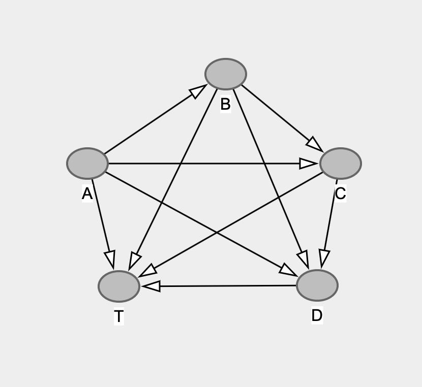
The DAG associated to this experiment is the following

Let us study association between $C$ and $T$. The d-separation criteria tells us that in this BN, without conditioning on any variable all the paths from $C$ to $T$ are open and I expect that, by closing some of them, the dependency between $C$ and $T$ decreases. In this particular graph, we expect the dependence by conditioning on $\{A,D\}$ to be higher than the one obtained by conditioning on $\{A,B,D\}$ since the latter case blocks $T\leftarrow B \rightarrow C$ as well as the paths through $A$ and $D$. Putting this in formulas, we expect to see

$dep(C,T|\{A,D\}) > dep(C,T|\{A,B,D\})$

By using the negative p-value as a dependence measure (as suggested here) these assumptions are violated since the R code outputs

$dep(C,T|\{A,D\}) = -pvalue_{C\perp T|\{A,D\}} = -1.78*10^{-09}$

$dep(C,T|\{A,B,D\}) = -pvalue_{C\perp T|\{A,B,D\}}= -1.52*10^{-11}$

therefore

$dep(C,T|\{A,D\}) < dep(C,T|\{A,B,D\})$

Any idea why this happens? May that be that the p-values (and the negative p-values as well) are not suited for studying dependency comparisons as the one I did?

Here's the code for this example

library(bnlearn)
set.seed(120395)

A = rnorm(n = 100, mean = 0, sd = sqrt(1))
B = A + rnorm(n = 100, mean = 0, sd = sqrt(1))
C = A + B + rnorm(n = 100, mean = 0, sd = sqrt(1))
D = A + B + C + rnorm(n = 100, mean = 0, sd = sqrt(1))
T = A + B + C + D + rnorm(n = 100, mean = 0, sd = sqrt(1))

df <- data.frame(A, B, C, D, T)

t1 <- ci.test("C", "T", data = df, test = "cor")
t2 <- ci.test("C", "T", "A", data = df, test = "cor")
t3 <- ci.test("C", "T", "B", data = df, test = "cor")
t4 <- ci.test("C", "T", "D", data = df, test = "cor")
t5 <- ci.test("C", "T", c("A","B"), data = df, test = "cor")
t6 <- ci.test("C", "T", c("A","D"), data = df, test = "cor")
t7 <- ci.test("C", "T", c("B","D"), data = df, test = "cor")
t8 <- ci.test("C", "T", c("A","B","D"), data = df, test = "cor")
print(c(t1$p.value, t2$p.value, t3$p.value, t4$p.value, 
        t5$p.value, t6$p.value, t7$p.value, t8$p.value))

Output:

[1] 5.008861e-67 2.379113e-42 2.425548e-32 6.708171e-09 2.204601e-25
[6] 1.783842e-09 1.329351e-09 1.521039e-11

Answer 1

Any idea of why this happens?

You start your reasoning by stating that you would expect the statistical dependence between B and T given A (a confounder) to be smaller than the statistical dependence between B and T, that is: $I(B;T) > I(B;T|A)$, being $I$ the Mutual Information. Yes, you're right, it should. And it does. See the code below (based on the code you shared).

set.seed(120395)
A = rnorm(n = 100, mean = 0, sd = sqrt(1))
B = A + rnorm(n = 100, mean = 0, sd = sqrt(1))
T = A + B + rnorm(n = 100, mean = 0, sd = sqrt(1))    

miic::discretizeMutual(B,T, plot=FALSE)$info
0.7031494
miic::discretizeMutual(B,T, matrix_u=matrix(A), plot=FALSE)$info
0.2519784

The issue here is that you're confusing the statistical significance of the independence test with the effect size of the dependence. Even with your independence test, if you check the objects t1 and t2, you will see that you find a Pearson correlation of $0.89$ at first, and then $0.76$ after adjusting for the confounder. So your own simulation shows what you expected, which is indeed correct.

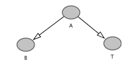
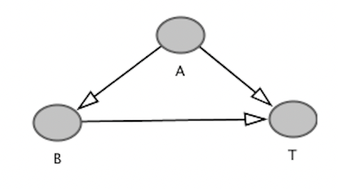
Regarding the p-values, you can inspect the objects returned by the ci.test function and you will see that what your p-values are suggesting that there is no independence, in any case. That's actually something that just now I noticed: Even though you mention d-separation in the title of your question, there is no d-separation in your question. You're confusing two different graphs. You probably think that the DAG you described through your three structural equations is the one below:

That is, $B$ and $T$ are independent but are observed to be dependent due to the confounding effect of $A$. You do not need to add the + B in the $T$ to have the spurious dependence, it's already there because both are caused by $A$. However, your structural equations led to the causal diagram below:

That is, $B$ and $T$ are dependent. And though you can decrease the dependence between them by adjusting for $A$, a confounding factor, you can not d-separate them, because they're directly dependent. It's the opposite, they're d-connected. That's why both p-values suggest a lack of independence. Besides, the first one being larger does not surprise me, since there is even less evidence that they are independent. By adjusting for a confounder, you decrease the dependence, and therefore make it less unlikely to be independent.

May that be because the probability distribution of the variables is not faithful to the DAG as pointed in the answer here?

No, because you made it faithful. You could create a set of structural equations and "hide" part of it, or create the relationships in a way that you would create non structural independencies (canceling pathways). However, that's not what you did. You made it pretty clear that $A$ causes $B$ and $T$, and $B$ causes $T$. Cinelli wrote some comments about that here.