R- empirical critical value in t-test

Question

I have the following assignment with R:

Simulate 5000 samples of size 15 from the distribution chi.sq with df=5. For each of these samples do the test H0: 𝜇 = 5 vs 𝐻1: 𝜇 <5 with alpha 3%, using the t-test for the mean of a normal population. Next, estimate the exact alpha of the test (ie find the percentage of incorrect rejections of H0). Is it close to 3%? If you had to "correct" the critical value you used in (a), what would it be? Hint: Use 𝑡 = (𝑋̅ - 𝜇0) √𝑛 as a statistical control function and find (by simulation) its distribution when the data comes from the chi square distribution(df=5). Then select an appropriate quantile of this distribution as the critical control point.

My attempt so far:

 sims<-2000
 alpha<-0.03
 n<-15

 mu1<-5

 X<-matrix(rchisq(n*sims,mu1),ncol=sims,nrow=n)
 
 xbars<-apply(X,2,mean)
 stdevs<-apply(X,2,sd)
 
 testTs<-(xbars-mu1)/(stdevs/sqrt(n))
 
 
 hist(testTs,xlim=c(-4,4),col="salmon",xlab="",probability=T,
        ylim=c(0,0.5),main="")
 
 
 Ucrit<-qt(1-alpha,df=(n-1))
 Lcrit<-qt(alpha,df=(n-1))
 
 xs<-seq(-4,4,by=0.05)
 ys<-dt(xs,df=(n-1))

  lines(xs,ys,lwd=2,col="red")
  lines(c(-4,4),c(0,0),lwd=3)
  lines(c(Lcrit,Lcrit),c(0,dt(Lcrit,df=(n-1))),lwd=2)
  lines(c(Ucrit,Ucrit),c(0,dt(Ucrit,df=(n-1))),lwd=2)
  
  SPU<-length(testTs[testTs>Ucrit])/length(testTs)
  SPL<-length(testTs[testTs<Lcrit])/length(testTs)
  simPower<-SPU+SPL
  simPower

Many thanks for your time!

Answer 1

First, experiment with (appropriate) normal data to show that the significance level is truly 3%. I use more than 5000 iterations to get better accuracy; $10^5$ iterations are enough to get about 2-place accuracy.

set.seed(1217) # for reproducibility
t.stat = replicate(10^5, t.test(rnorm(15,5,10), mu=5, alt="less")$stat)
mean(t.stat <= qt(.03, 14))
[1] 0.03034   ​# aprx sig level, normal data
2*sd(t.stat <= qt(.03, 14))/sqrt(10^5)
[1] 0.0010848 # aprx 95% margin of simulation error

The true significance level is $0.030 \pm 0.001.$ The critical value for a test at the 3% level, from distribution $\mathsf{T}(\nu = 14),$ is $c = -2.0461.$

qt(.03, 14)
[1] -2.046169

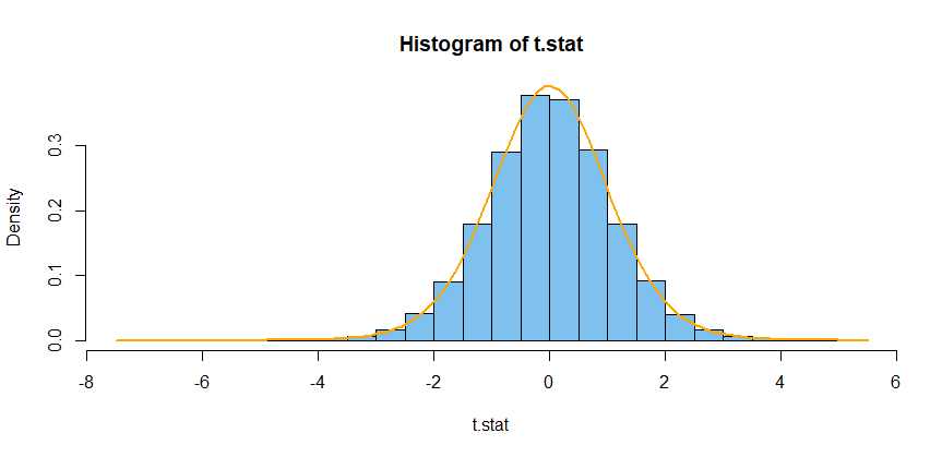
Below is a plot of the $10^5$ t statistics along with the density function of $\mathsf{T}(\nu=14)$

hist(t.stat, prob=T, br=30, col="skyblue2")
 curve(dt(x, 14), add=T, lwd=2, col="orange")

Repeat for (inappropriate) chi-squared data.

set.seed(1218) # for reproducibility     
t.stat = replicate(10^5, t.test(rchisq(15,5), mu=5, alt="less")$stat)
mean(t.stat <= qt(.03, 14))
[1] 0.06346      # aprx sig level, normal data 
2*sd(t.stat <= qt(.03, 14))/sqrt(10^5)
[1] 0.001541862

With such severely non-normal data, the true significance level is $0.063 \pm 0.002,$ which is far from 3%.

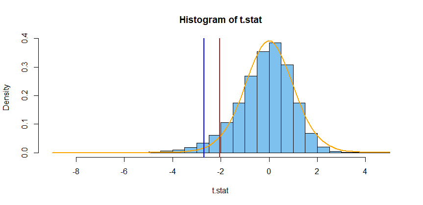
The critical value $c^\prime$ that cuts probability 3% from the lower tail of the distribution of the t-statistic used just above is approximately $-2.703.$

quantile(t.stat, .03)
       3% 
-2.702873 

Here is a plot of the t statistics from using chi-squared data along with the density function of $\mathsf{T}(\nu=14).$ It is clear that the t statistic for such chi-squared data does not have a t distribution.

The critical value $c$ that cuts 3% from the lower tail of the t distribution is shown as a brown line; the value $c^\prime$ that cuts 3% from the lower tail of the simulated values in the histogram is shown in blue.

Using this modified critical value, the significance level for the t statistic with such chi-squared data is about 3%.

> mean(t.stat <= -2.703)
[1] 0.03