1
$\begingroup$

I know that this question was already posed several times but I am not sure If I really got the interpretation for spline functions right.

I have an ordered model that is regressed on an index ranging from ca. 0.028 to 0.42 for which I created a natural spline with splines::ns(X, 3).

Below you can see an example from the "housing" dataset with the variable Freq. If I look at the modelsummary I get three coefficients for ns(Freq, 3). When looking at the information from ns(Freq, 3) I get two boundary knots and two inner knots. Thus I'd interpret the coefficients as: When Freq<Knot_1 an 1 unit increase in Freq increases the probability for satisfation == High c.p. on average by 0.75... But if I use ggpredict and calculate slopes between the boundaries (dashed lines) I don't come to the same numbers.

So question:

Is it right to interpret the coefficients like I did, and: are the higher coefficients (ns(X,3)2 and ns(X,3)3) all relative to the baseline (outer knot_low) or relative to the last knot?

EXAMPLE:

> housing %>% glimpse
Rows: 72
Columns: 5
$ Sat  <ord> Low, Medium, High, Low, Medium, High, Low, Medium, High, Low, Medium, High, Low, Medium, High, Low, Medium, High, Low…
$ Infl <fct> Low, Low, Low, Medium, Medium, Medium, High, High, High, Low, Low, Low, Medium, Medium, Medium, High, High, High, Low…
$ Type <fct> Tower, Tower, Tower, Tower, Tower, Tower, Tower, Tower, Tower, Apartment, Apartment, Apartment, Apartment, Apartment,…
$ Cont <fct> Low, Low, Low, Low, Low, Low, Low, Low, Low, Low, Low, Low, Low, Low, Low, Low, Low, Low, Low, Low, Low, Low, Low, Lo…
$ Freq <int> 21, 21, 28, 34, 22, 36, 10, 11, 36, 61, 23, 17, 43, 35, 40, 26, 18, 54, 13, 9, 10, 8, 8, 12, 6, 7, 9, 18, 6, 7, 15, 1…
> 
> # ##get knots information
> # ns(housing$Freq,3)
> # attr(,"degree")
> # [1] 3
> # attr(,"knots")
> # 33.33333% 66.66667% 
> #        13        23 
> # attr(,"Boundary.knots")
> # [1]  3 86
> # attr(,"intercept")
> # [1] FALSE
> # attr(,"class")
> # [1] "ns"     "basis"  "matrix"
> 
> tibble( Knots = c("out_low", "inner_1", "inner_2", "out_high"), 
+         Val = c(3,13,23,86 ))-> splinetab
> splinetab
# A tibble: 4 × 2
  Knots      Val
  <chr>    <dbl>
1 out_low      3
2 inner_1     13
3 inner_2     23
4 out_high    86
> #
> clm(Sat ~ ns(Freq, 3), data = housing) %>% S
formula: Sat ~ ns(Freq, 3)
data:    housing

 link  threshold nobs logLik AIC    niter max.grad cond.H 
 logit flexible  72   -77.98 165.96 3(0)  4.96e-08 1.6e+02

Coefficients:
             Estimate Std. Error z value Pr(>|z|)
ns(Freq, 3)1   0.7342     1.1112   0.661    0.509
ns(Freq, 3)2   2.1358     1.7693   1.207    0.227
ns(Freq, 3)3   0.5048     1.5248   0.331    0.741

Threshold coefficients:
            Estimate Std. Error z value
Low|Medium    0.2328     0.7435   0.313
Medium|High   1.6539     0.7687   2.152
> 
> #
> ggeffect(clm(Sat ~ ns(Freq, 3), data = housing), terms = "Freq [3,13,23,86]") %>% filter(response.level == "High")-> ge
> ge
# Predicted probabilities of Sat

Freq | Predicted |       95% CI
-------------------------------
   3 |      0.16 | [0.04, 0.46]
  13 |      0.34 | [0.20, 0.52]
  23 |      0.39 | [0.25, 0.54]
  86 |      0.35 | [0.03, 0.91]
> #
> ggplot(ge, aes(x= x, y = predicted))+geom_smooth()+geom_vline(aes(xintercept = 3), lty = 3)+geom_vline(aes(xintercept = 13), lty = 3)+geom_vline(aes(xintercept = 23), lty = 3)+geom_vline(aes(xintercept = 86), lty = 3)
`geom_smooth()` using method = 'loess' and formula 'y ~ x'

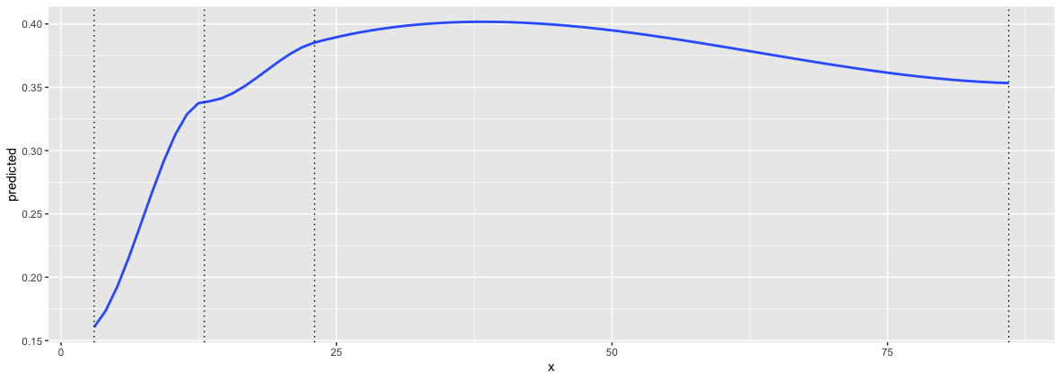
enter image description here

$\endgroup$

1 Answer 1

1
$\begingroup$

Is it right to interpret the coefficients like I did, and: are the higher coefficients (ns(X,3)2 and ns(X,3)3) all relative to the baseline (outer knot_low) or relative to the last knot?

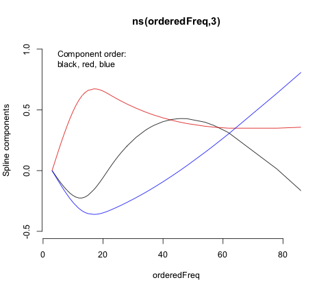
There is no simple heuristic interpretation of spline-term coefficients, particularly when ns() is used. The coefficients have to be interpreted in terms of how the spline is expressed in the model matrix for the regression. The ns() function uses a B-spline basis of orthogonal polynomials, leading to the following with the example data.

library(splines)
library(MASS) ## for housing data
## put the "Freq" values into ascending order 
orderedFreq <- housing$Freq[order(housing$Freq)]
mmNS <- model.matrix(~ ns(orderedFreq, 3))
plot(mmNS[,2]~orderedFreq,type="l",bty="n",ylab="Spline components",ylim=c(-0.5,1))
lines(mmNS[,3]~orderedFreq,type="l",col="red")
lines(mmNS[,4]~orderedFreq,type="l",col="blue")
title(main="ns(orderedFreq,3)")

ns() spline

I think that illustrates the futility of trying for a simple interpretation of the corresponding regression coefficients.

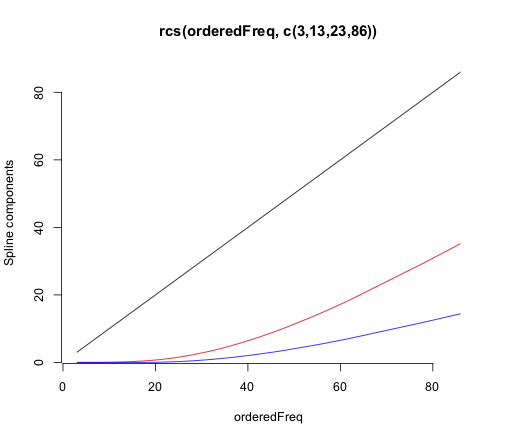
The rcs() function in the rms package comes closer to what you want. It uses a different spline basis, resulting in the following for these data:

library(rms)
mmRCS <- model.matrix(~ rcs(orderedFreq, c(3,13,23,86))) ## to match knots chosen by ns()
plot(mmRCS[,2]~orderedFreq,type="l",bty="n")
lines(mmRCS[,3]~orderedFreq,type="l",col="red")
lines(mmRCS[,4]~orderedFreq,type="l",col="blue")
title(main="rcs(orderedFreq, c(3,13,23,86))")

rcs() spline

This starts with a simple linear term and adds nonlinear terms. Section 2.4 of Frank Harrell's course notes goes into the details of this spline basis. As he explains in this answer, this leads more naturally to expression of the model in terms of an equation, which can be shown via the Function() function in the rms package. Also, unlike ns(), rcs() doesn't by default place the outermost knots at the outermost data points.

I think of interpreting individual spline-term coefficients as a "don't try this at home" type of thing, unless you really know what you're doing. Use built-in prediction functions to document the shape and confidence intervals of the associations of the continuous predictor with outcome.

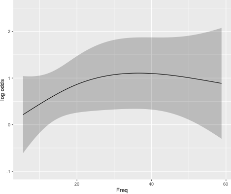
To illustrate, here's a proportional odds model built with rms tools. Note that those tools are designed to work with each other, so you can't just apply them to your clm() model. This doesn't exactly match your model, as it doesn't put knots at the extremes and it models exceedance probabilities.

ddHousing <- datadist(housing) 
options(datadist="ddHousing") ## sets up a datadist to simplify later use of Predict
lrmMod <- lrm(Sat~rcs(Freq,3),data=housing)
ggplot(Predict(lrmMod))

predicted log odds

Function() produces an R function for the linear predictor of the model. You'll notice that the pmax() terms show the changes of the function at each of the knot locations.

lrmFunction <- Function(lrmMod)
lrmFunction
##function(Freq = 19.5) {+0.05079445* Freq-3.1467476e-05*pmax(Freq-6,0)^3+4.2795767e-05*pmax(Freq-19.5,0)^3-1.1328291e-05*pmax(Freq-57,0)^3 }
##<environment: 0x7fa627d9c368>

You can get Latex code for the model with latex(lrmMod), which provides the following after a bit of adjustment into MathJax.

$$ {\rm Prob}\{{\rm Sat}\geq j\} = \frac{1}{1+\exp(-\alpha_{j}-X\hat\beta)}, {\rm \ \ where} \\ \begin{eqnarray*} \hat{\alpha}_{\rm Medium} &=&-0.06570302\\ \hat{\alpha}_{\rm High} &=&-1.48320190\\ \end{eqnarray*} $$ $$ {X\hat{\beta}=}\\ + 0.05079445 {\rm Freq}-3.146748\!\times\!10^{-5}({\rm Freq}-6)_{+}^{3}+4.279577\!\times\!10^{-5 }({\rm Freq}-19.5)_{+}^{3} \\ -1.132829\!\times\!10^{-5}({\rm Freq}-57)_{+}^{3} \\ \text{and} \left((x)_{+}=x \text{ if } (x > 0), 0 \text{ otherwise}\right).\\ $$

$\endgroup$
9
  • $\begingroup$ FOA thank you. I thought something like this... I also went through the course notes and his boot (...not in detail for time reasons...). BTW the book link.springer.com/book/10.1007/978-3-319-19425-7 is really great! I tried the orm function but could not enter weights (I have survey data with weights). Do you know about an option for that? And also I couldn't find this Function() function... $\endgroup$
    – Eco007
    Commented Mar 27, 2022 at 6:56
  • $\begingroup$ I went through the book but I still don't get the "Formula" of my model. What would be the interpretation of the restricted cubic splines? $\endgroup$
    – Eco007
    Commented Mar 27, 2022 at 7:54
  • $\begingroup$ @Eco007 I added examples for Predict() and Function() with the lrm() function, which allows for case weights and ordinal regression. The orm() function is designed more for modeling continuous outcomes via proportional odds. Both ns() and rcs() use restricted cubic splines, which are "restricted" in that the functions are linear beyond the outer knots. That's hard to tell with ns() as its default outermost knots are at the limits of the values. Those two functions use different spline bases and default knot locations. $\endgroup$
    – EdM
    Commented Mar 27, 2022 at 15:22
  • $\begingroup$ :-) Thanks a lot!! So only few questions: the $(x)_+ = x \ \text{for}\ x>0$ stands for the linearity in $x$? here I get two coefficients rcs(x, 3) and rcs(x,3)'. The latter is the first derivative of the spline function? And would you advise to use the rcs function within a clm model? When I use interactions terms together with the spline it tells me anyway that the model is unidentifiable because of too large eigenvalues... $\endgroup$
    – Eco007
    Commented Mar 27, 2022 at 21:17
  • 1
    $\begingroup$ @Eco007 that $(x)_+$ form (or pmax(x,0) in the lrmFunction) represents a step change in the equation when the argument $x$ exceeds 0. In the full equation there are several such arguments (like in $(\text{Freq}-6)_+$, where $x=\text{Freq}-6$) representing whether the predictor value has exceeded one or more of the knots. All those terms here, however, are cubic terms. The rcs(x,3) coefficient is for the linear component of the spline fit, but the '/'' indicators from rcs() don't represent derivatives, just higher-level non-linear terms. Don't try to interpret them individually. $\endgroup$
    – EdM
    Commented Mar 27, 2022 at 21:37

Your Answer

By clicking “Post Your Answer”, you agree to our terms of service and acknowledge you have read our privacy policy.

Not the answer you're looking for? Browse other questions tagged or ask your own question.