Should I use a Simple Linear or Logistic Regression

Question

I have this reproducible dataset:

structure(list(age = c(62.84998, 60.33899, 52.74698, 42.38498, 
 79.88495, 93.01599, 62.37097, 86.83899, 85.65594, 42.25897), 
     death = c(0, 1, 1, 1, 0, 1, 1, 1, 1, 1), sex = c("male", 
     "female", "female", "female", "female", "male", "male", "male", 
     "male", "female"), hospdead = c(0, 1, 0, 0, 0, 1, 0, 0, 0, 
     0), slos = c(5, 4, 17, 3, 16, 4, 9, 7, 12, 8), d.time = c(2029, 
     4, 47, 133, 2029, 4, 659, 142, 63, 370), dzgroup = c("Lung Cancer", 
     "Cirrhosis", "Cirrhosis", "Lung Cancer", "ARF/MOSF w/Sepsis", 
     "Coma", "CHF", "CHF", "Lung Cancer", "Colon Cancer"), dzclass = c("Cancer", 
     "COPD/CHF/Cirrhosis", "COPD/CHF/Cirrhosis", "Cancer", "ARF/MOSF", 
     "Coma", "COPD/CHF/Cirrhosis", "COPD/CHF/Cirrhosis", "Cancer", 
     "Cancer"), num.co = c(0, 2, 2, 2, 1, 1, 1, 3, 2, 0), edu = c(11, 
     12, 12, 11, NA, 14, 14, NA, 12, 11), income = c("$11-$25k", 
     "$11-$25k", "under $11k", "under $11k", NA, NA, "$25-$50k", 
     NA, NA, "$25-$50k"), scoma = c(0, 44, 0, 0, 26, 55, 0, 26, 
     26, 0), charges = c(9715, 34496, 41094, 3075, 50127, 6884, 
     30460, 30460, NA, 9914), totcst = c(NA_real_, NA_real_, NA_real_, 
     NA_real_, NA_real_, NA_real_, NA_real_, NA_real_, NA_real_, 
     NA_real_), totmcst = c(NA_real_, NA_real_, NA_real_, NA_real_, 
     NA_real_, NA_real_, NA_real_, NA_real_, NA_real_, NA_real_
     ), avtisst = c(7, 29, 13, 7, 18.666656, 5, 8, 6.5, 8.5, 8
     ), race = c("other", "white", "white", "white", "white", 
     "white", "white", "white", "black", "hispanic"), sps = c(33.8984375, 
     52.6953125, 20.5, 20.0976562, 23.5, 19.3984375, 17.296875, 
     21.5976562, 15.8984375, 2.2998047), aps = c(20, 74, 45, 19, 
     30, 27, 46, 53, 17, 9), surv2m = c(0.262939453, 0.0009999275, 
     0.790893555, 0.698974609, 0.634887695, 0.284973145, 0.892944336, 
     0.670898438, 0.570922852, 0.952880859), surv6m = c(0.0369949341, 
     0, 0.664916992, 0.411987305, 0.532958984, 0.214996338, 0.820922852, 
     0.498962402, 0.24899292, 0.887939453), hday = c(1, 3, 4, 
     1, 3, 1, 1, 1, 1, 1), diabetes = c(0, 0, 0, 0, 0, 0, 0, 1, 
     0, 0), dementia = c(0, 0, 0, 0, 0, 0, 0, 0, 1, 0), ca = c("metastatic", 
     "no", "no", "metastatic", "no", "no", "no", "no", "metastatic", 
     "metastatic"), prg2m = c(0.5, 0, 0.75, 0.899999619, 0.899999619, 
     0, NA, 0.799999714, 0.049999982, NA), prg6m = c(0.25, 0, 
     0.5, 0.5, 0.8999996, 0, 0.6999998, 0.3999999, 0.0001249999, 
     NA), dnr = c("no dnr", NA, "no dnr", "no dnr", "no dnr", 
     "no dnr", "no dnr", "no dnr", "dnr after sadm", "no dnr"), 
     dnrday = c(5, NA, 17, 3, 16, 4, 9, 7, 2, 8), meanbp = c(97, 
     43, 70, 75, 59, 110, 78, 72, 97, 84), wblc = c(6, 17.0976562, 
     8.5, 9.09960938, 13.5, 10.3984375, 11.6992188, 13.5996094, 
     9.69921875, 11.2988281), hrt = c(69, 112, 88, 88, 112, 101, 
     120, 100, 56, 94), resp = c(22, 34, 28, 32, 20, 44, 28, 26, 
     20, 20), temp = c(36, 34.59375, 37.39844, 35, 37.89844, 38.39844, 
     37.39844, 37.59375, 36.59375, 38.19531), pafi = c(388, 98, 
     231.65625, NA, 173.3125, 266.625, 309.5, 404.75, 357.125, 
     NA), alb = c(1.7998047, NA, NA, NA, NA, NA, 4.7998047, NA, 
     NA, 4.6992188), bili = c(0.19998169, NA, 2.19970703, NA, 
     NA, NA, 0.39996338, NA, 0.39996338, 0.19998169), crea = c(1.19995117, 
     5.5, 2, 0.79992676, 0.79992676, 0.69995117, 1.59985352, 2, 
     1, 0.79992676), sod = c(141, 132, 134, 139, 143, 140, 132, 
     139, 143, 139), ph = c(7.459961, 7.25, 7.459961, NA, 7.509766, 
     7.65918, 7.479492, 7.509766, 7.449219, NA), glucose = c(NA_real_, 
     NA_real_, NA_real_, NA_real_, NA_real_, NA_real_, NA_real_, 
     NA_real_, NA_real_, NA_real_), bun = c(NA_real_, NA_real_, 
     NA_real_, NA_real_, NA_real_, NA_real_, NA_real_, NA_real_, 
     NA_real_, NA_real_), urine = c(NA_real_, NA_real_, NA_real_, 
     NA_real_, NA_real_, NA_real_, NA_real_, NA_real_, NA_real_, 
     NA_real_), adlp = c(7, NA, 1, 0, NA, NA, 0, NA, NA, 0), adls = c(7, 
     1, 0, 0, 2, 1, 1, 0, 7, NA), sfdm2 = c(NA, "<2 mo. follow-up", 
     "<2 mo. follow-up", "no(M2 and SIP pres)", "no(M2 and SIP pres)", 
     "<2 mo. follow-up", "no(M2 and SIP pres)", NA, NA, NA), adlsc = c(7, 
     1, 0, 0, 2, 1, 1, 0, 7, 0.4947999)), row.names = c(NA, 10L
 ), class = "data.frame")

I am wanting to obtain the proportions of male and female patients within the different races of the study patients. I used this code to get the proportions.

SB_xlsx11$sex_f = as.factor(SB_xlsx11$sex)
SB_xlsx11$race_f = as.factor(SB_xlsx11$race)
prop.table(table(SB_xlsx11$race_f, SB_xlsx11$sex_f))
##           
##                 female        male
##   asian    0.003530840 0.005185921
##   black    0.076133731 0.077347457
##   hispanic 0.014895730 0.017102505
##   other    0.005627276 0.006730663
##   white    0.336864173 0.456581706

I believe this is correct, as it separates male and female by race. I want to see if there is evidence to indicate that sex is associated with the race of the study patients. Would this be a simple linear regression or a simple logistic regression? I'm also feeling uncertain about which variable would be my predictor (x) and response (y) (y~x) if I want to see if sex is associated with race of study patients.

Answer 1

Poisson regression

What you could use is a Poisson regression. This would model the rate/counts for the number of patients occurring as a function of the predictor.

Linear or Logistic?

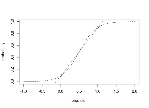
In the case when you only have a dummy variable (two values), then it does not matter whether you use a linear function or a logistic function.

In the plot below you see how it doesn't matter what sort of function you use when you only model only two values.

However, when you are looking at situations like age as a numeric predictor variable, then using some function as a logistic curve might give a difference.

In addition, for mixing two or more main effects there is an influence on the model depending on which function you use.

• In this case of Poisson regression, an exponential function (making the link function the inverse, a log-function) might work well. Then you model the outcome effectively as a multiplication of terms. E.g. the expected number of counts is modeled as a product of coefficients one for each main effect. An example of how the exponential function makes a multiplicative model is here.

Interaction term

I'm also feeling uncertain about which variable would be my predictor (x) and response (y) (y~x) if I want to see if sex is associated with race of study patients.

You would use an interaction term. The combination of both gender and race. Gender and race are both predictors of the response which is the count in the number of patients.

The result should be more or less the same as the $\chi^2$ test. The R-computation below demonstrates this

n = (2^6*3^4*5^2*11*283)
response = c(0.003530840, 0.005185921,
             0.076133731, 0.077347457,
             0.014895730, 0.017102505,
             0.005627276, 0.006730663,
             0.336864173, 0.456581706)*n
gender = rep(c("female", "male"),times = 5)
background = rep(c("asian", "black", "hispanic", "other", "white"), each = 2)

mod = glm(response ~ background * gender, family = poisson())
anova(mod, test = "Chisq")
# Analysis of Deviance Table
#
# Model: poisson, link: log
#
# Response: response
#
# Terms added sequentially (first to last)
#
#                   Df  Deviance Resid. Df Resid. Dev  Pr(>Chi)    
# NULL                                   9  759919240              
# background         4 752371092         5    7548148 < 2.2e-16 ***
# gender             1   6411572         4    1136576 < 2.2e-16 ***
# background:gender  4   1136576         0          0 < 2.2e-16 ***
# ---
# Signif. codes:  0 ‘***’ 0.001 ‘**’ 0.01 ‘*’ 0.05 ‘.’ 0.1 ‘ ’ 1


chisq.test(matrix(response,5,byrow=1))
#
# Pearson's Chi-squared test
# 
# data:  matrix(response, 5, byrow = 1)
# X-squared = 1142900, df = 4, p-value < 2.2e-16

The values of the $\chi^2$ statistic are close to each other for both methods, 1136576 and 1142900. The difference between the two methods is that the chi-squared test is considering the marginals, the totals of female/male and totals of backgrounds as, fixed and the Poisson regression does not.

Answer 2

Generally, when you have two categorical variables, you might want to use a Chi-square test. In R it would be something like:

chisq.test(x)

where x is your contingency table (e.g., x <- table(data$var1, data$var2)). This will test the association between the two variables.