Generalized additive model (gam) plot

Question

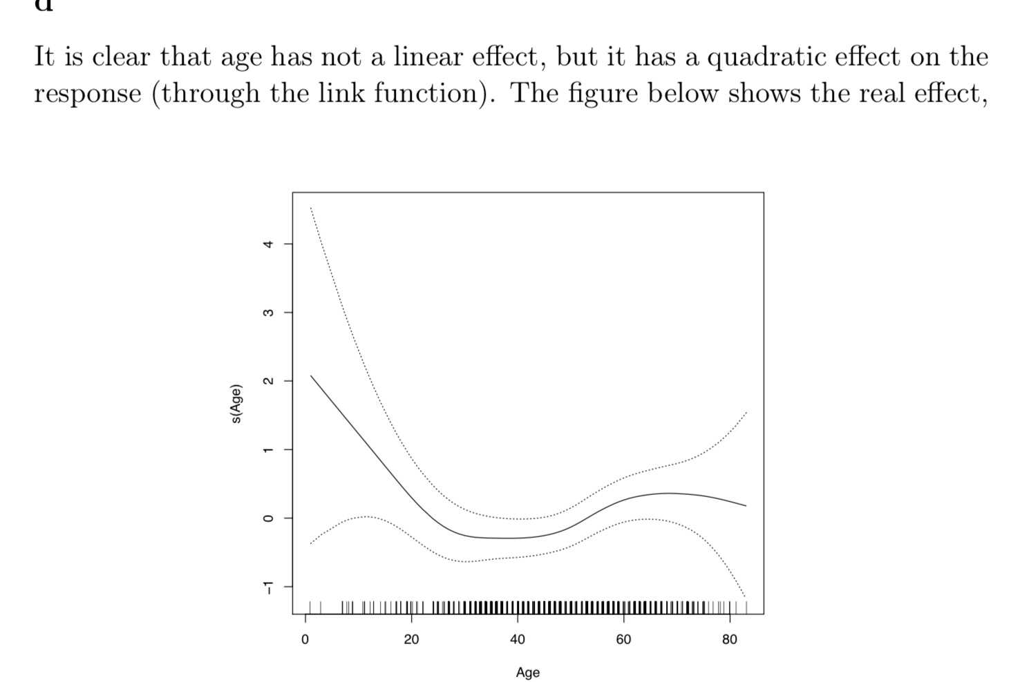
I got the following problem: If one would have fitted a generalised additive model allowing a smooth function to capture the effect of Age, which form would have it taken?

Call:
glm(formula = y ~ Age + I(Age^2) + Sex + Height + Weight,
family = binomial, data = data)
Coefficients:
          Estimate Std. Error z value Pr(>|z|)
(Intercept)  6.9060592  2.3973921   2.881  0.00397 **
Age         -0.0784407  0.0348305  -2.252  0.02432 *
I(Age^2)     0.0009048  0.0003630   2.493  0.01268 *
Sexfemale   -1.2326965  0.2539864  -4.853 1.21e-06 ***
Height      -0.0320293  0.0151363  -2.116  0.03434 *
Weight       0.0043771  0.0081598   0.536  0.59167
Null deviance: 620.27  on 449  degrees of freedom
Residual deviance: 579.00  on 444  degrees of freedom
AIC: 591

With this data we get the following plot

My question is: How do you manage to see that the plot will have that shape just by looking at the data we have been given? and which covariates do we look at? Are we just lokking at age-squared or age+age-squared?

Thanks for all the help I can get!

Answer 1

The result of glm that you posted includes Age and Age_squared as linear terms and we know from the significance of the squared term, that we need a squared term because things are not strictly linear.

The 'real effect' in the scan you posted is most likely the result of a GAM. In the GAM there is no point in including a squared term as the smoother is für more flexible/adaptable then the sum of a raw and a squared term.