Why do we need regularization for linear least squares given that a line is the simplest model possible?

Question

In linear least squares we are trying to fit a line to data. A line is the simplest model that can be fit to the data. How is it possible for a linear model to over-fit the data? In short why do we need regularization for fitting a line to a data?

I understand that regularization improves generalization performance ie over unseen datasets and reduces over-fitting to training data. But how would regularization reduce the over-fitting issue for a least complex model (i.e linear model)?

This question was posted on stackoverflow, was redirected here. Also asked on DataScience stackexchange, but I am yet to get any answers/comments on the same.

Answer 1

Great question! The need for regularization always depends on your sample size.

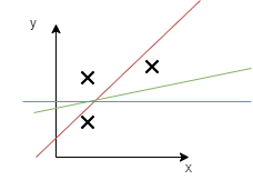
Imagine you do not have a lot of data, just three samples. I plotted three possible linear regression lines. The red one does not use regularization; for the green one, regularization on the slope parameter is used, and the blue regression has very strong regularization on the slope parameter.

Which one is the best model? We don't know. That will only become clear as more data is collected. But regularized models produce more conservative estimates, which often work better in practice.

That said, if you really only have the case of a simple linear regression (one input variable, like in my example), you will often have enough data to use an unregularized model.

But keep in mind that linear regression also works for multiple input variables. In that case, the model will have $p+1$ parameters if you have $p$ features. You need regularization if $p$ is large compared to your sample size.

In summary, a model is never a priori complex or simple, it always depends on the data you want to use the model for.

Answer 2

Another way of looking at it: A linear model is not the simplest model that can be fitted to the data - a linear model with a constraint on the values of the weights is even more simple. For example, if we constrain the number of non-zero weights, we have a model that is structurally less complex - it has fewer parameters. As we increase the number of non-zero weights, we create a sequence of nested models of increasing complexity. A model with three non-zero weights can do everything a model with two non-zero weights can do, and also a few things it can't, so it must be a more complex model in some sense.

We can do something similar with regularisation, but it is a bit more subtle. We can create another sequence of models of increasing complexity by putting a constraint on the norm of the weight vector (limiting the magnitude of the weights rather than the number of non-zero weights). We then have an optimisation problem of the form:

$\mathrm{min}_\vec{\theta} f(\vec{\theta}) \quad \mathrm{s.t.} \quad \|\vec{\theta}\|^2 < C$

where $\vec{\theta}$ is the vector of model parameters (weights) and $C$ is the hyper-parameter controlling the maximum allowed value of the norm of the parameter vector and $f(\cdot)$ is the loss function (e.g. sum of squares). If we have a model with a particular value of $C$ and then increase $C$ a bit (to $C'$), then it can do anything it previously could, but it can also realize some additional mappings that it couldn't before. So as we increase $C$, we create models that are potentially more and more complex.

How does this relate to regularisation? One way of solving a constrained optimisation problem is to take the Lagrangian to turn it into an unconstrained optimisation problem, and in this case, the Lagrangian is:

$\Lambda(\vec{\theta},\lambda) = f(\vec{\theta}) + \lambda\|\vec{\theta}\|^2 - \lambda C.$

We can ignore the last term as it doesn't depend on the parameter vector, and what is left is a regularised loss function.

So we see that regularisation is a way of controlling the complexity of even a linear model, by limiting the set of mappings it can implement.

If we think of one-dimensional regression tasks, it is difficult to find a lot of value in regularisation, but when we have models with lots of parameters, regularisation becomes more obviously useful. Some of the attributes may be correlated with the target by random chance and have no predictive value. Regularisation will help surprress those attributes, and result in a model with better generalsiation.

Modelling data generally involved fitting the complexity of the model (class) to the complexity of the data we have available, and regularisation provides a convenient way of doing that (it is a continuous hyper-parameter, so it is a bit less of a blunt instrument that e.g. feature selection).

Just to add, I've been a bit vague with terminology here. Really is is nested sets of model/hypothesis classes rather than models, i.e. the set of models that could be realised within the constraint imposed by the value of the regularisation parameter (c.f. @Ben's answer).

Answer 3

I think part of the misunderstanding may be driven by the meaning of "model". A linear model is a set of distributions, where (for simplicity) we can consider that each distribution is represented by a line. Thus a linear model is a set (or collection) of lines - not a single line. The bigger that set is, the more complex the model is. Regularization--like removing variables from a regression--reduces the complexity of the model by making the model contain fewer lines. This can be helpful since more complex models can be more prone to overfitting.

Answer 4

There is an elegant theoretical reason one might want to regularize a linear model. It is related to Dikran's answer, in that we are expressing an assumption about the weights. In essence, L2 regularization applied to a least squares linear fit expresses a Gaussian prior assumption on weight space. I'll show below the broad strokes of M-estimators used to derive two things:

• (MLE) Assume Gaussian distributed observation noise $\implies$ least squares loss gives maximum likelihood model.
• (MAP) Assume Gaussian distribution of model weights $\implies$ L2 regularization on loss gives maximum likelihood model.

I'll leave out details for brevity, since they are available broadly already. The point is that MSE loss and L2 regularization can be derived from first principles and simple distributional assumptions.

MLE from observation noise

In the linear regression setting, we learn model weights $\mathbf{w}$ to make scalar predictions $\hat{y}$ from samples $\mathbf{x}$ as

$$ \hat{y} = \mathbf{w}^T\mathbf{x} $$

When one assumes the true underlying distribution is a linear combination and a Gaussian noise term,

$$ y|\mathbf{x} = \mathbf{w}^T \mathbf{x} + \mathcal{N}(0, \sigma^2) $$

then maximum likelihood estimation (MLE) induces a mean squared error loss

$$ \mathcal{L}_{MLE}(\mathbf{w}) = \sum_{i=1}^n (\mathbf{w}^T\mathbf{x}_i - y)^2 $$

such that minimizing $\mathcal{L}_{MLE}$ produces the MLE estimate of weights.

MAP from weight distribution

Further, if one assumes a Gaussian prior distribution on the model weights $\mathbf{w}$ with each weight $w_i$ having identical variance $\nu^2$

$$ w_i \sim \mathcal{N}(0, \nu^2) $$

then the analogous maximum a posteriori (MAP) estimation induces the L2 regularizer with regularization weight $\lambda = \frac{\sigma^2}{\nu^2}$

$$ \mathcal{L}_{MAP}(\mathbf{w}) = \sum_{i=1}^n (\mathbf{w}^T\mathbf{x}_i - y)^2 + \lambda||\mathbf{w}||^2_2 $$

such that minimizing $\mathcal{L}_{MAP}$ produces the MAP estimate of weights.

So choosing least squares loss expresses a Gaussian observation noise assumption. And choosing L2 regularization expresses a Gaussian model weight assumption, where $\lambda$ expresses an assumed variance ratio between observation noise and model weights.