Contrast of contrasts emmeans how to properly represent interaction effect

Question

I've tried to custom code contrasts in emmeans to understand the effect of a combined treatment variable (combination of factors, Dose_Climate). I am not sure the contrast of contrasts I've coded is properly capturing the same thing as a regular interaction effect (which is what I want) because I have unexpected results from the contrast of contrasts.

The variable was combined because models with the interaction Dose*Climate had high vifs and thus I was worried about type-ii error (p-values for interaction effect didn't make sense when looking at the data).

#data
Row <- c("A","A","A","A","A","A","B","B","B","B","B","B","C","C","C","C","C","C","D","D","D","D","D","D","E","E","E","E","E","E","F","F","F","F","F","F")
Dose_Climate <-c("H_1Normal","H_Climate","2L_1Normal","2L_Climate","1K_1Normal","1K_Climate","1K_1Normal","H_Climate","H_1Normal",
"2L_Climate","2L_1Normal","1K_Climate","2L_Climate","1K_1Normal","1K_Climate","H_1Normal","H_Climate","2L_1Normal",
"H_1Normal","2L_Climate","2L_1Normal","1K_Climate","1K_1Normal","H_Climate","1K_1Normal","H_1Normal","H_Climate",
"2L_1Normal","2L_Climate","1K_Climate","2L_Climate","H_Climate","H_1Normal","2L_1Normal","1K_Climate","1K_1Normal")
Pest <- c(0,3,2,2,12,4,5,4,0,0,5,7,0,8,3,1,2,1,0,1,1,4,9,2,6,1,3,0,7,10,2,1,1,2,6,5)
df <- data.frame(Row, Dose_Climate, Pest)

#model
m1 <- bglmer(Pest~Dose_Climate+(1|Row), data=df,
             family = poisson) #using blme because of singularity issues
#custom contrast set to answer research questions
emm <- emmeans(m1, ~Dose_Climate)
H_Climate = c(0,0,0,0,0,1) # translating the order into a matrix
H_Normal = c(0,0,0,0,1,0)
K_Climate = c(0,1,0,0,0,0)
K_Normal = c(1,0,0,0,0,0)
L_Climate = c(0,0,0,1,0,0)
L_Normal = c(0,0,1,0,0,0)
c1 <- contrast(emm, method=list("K_Normal-L_Normal"=K_Normal-L_Normal,
                                "K_Normal-H_Normal"=K_Normal-H_Normal,
                                "L_Normal-H_Normal"=L_Normal-H_Normal,
                                "K_Climate-L_Climate"=K_Climate-L_Climate,
                                "K_Climate-H_Climate"=K_Climate-H_Climate,
                                "L_Climate-H_Climate"=L_Climate-H_Climate),
               adjust="Holm")
c1

If you run the code, from the set we see that the first three contrasts are similar to the second three in that K vs L is significant and K vs H is significant but L vs H is not. Here I would not expect a significant interactions contrast because the relationships between the individual levels are similar within the "Normal" set and the "Climate" set. But..

Normal= c(1,1,1,0,0,0) #coding position of Normal in c1 grid object
Climate= c(0,0,0,1,1,1) #coding position of Climate in c1 grid object
c2 <- contrast(c1, method=list("Normal-Climate"=Normal-Climate)) 
c2

The contrast of the contrasts is significant. This wasn't expected (and other models of mine have also shown unexpected contrast of contrasts behavior with this coding). Am I properly representing an interaction effect with this coding? As I understand it, my code takes an "average difference" so to speak over the first three contrasts and compares it with the "average difference" from the second three contrasts. I am just not sure if this is comparable to testing for an interaction, and if not, what the proper coding for it would be. Thanks in advance.

Answer 1

First, as Russ Lenth said in comments, it's best to work with stuff that's already been set up. What you have is a simple interaction model, so set this up as an interaction. To rework your data for that, I did:

df[,"Dose"] <- sub("(.*)_.*","\\1",df$Dose_Climate)
df[,"Climate"] <- sub(".*_(.*)","\\1",df$Dose_Climate)
df$Dose <- factor(df$Dose)
df$Climate <- factor(df$Climate)
df$Row <- factor(df$Row)

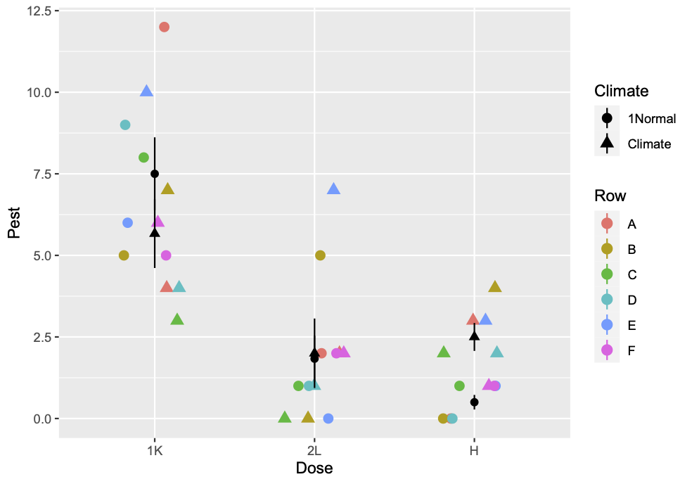
Second, look at your data

library(ggplot2)
ggplot(df,mapping=aes(x=Dose,y=Pest,shape=Climate,color=Row)) +
    geom_jitter(cex=3,height=0,width=0.2) + 
    stat_summary(data=df,mapping=aes(x=Dose,y=Pest,group=Climate),
    fun.data=mean_se)

Third, it's thus not clear just what you mean by

what I'm aiming for ... is an overall Climate-Normal contrast of the 3 dose contrasts within Climate and Normal

or if that would even be a fair representation of your data. Although you seem focused on L vs H differences not being significant within either value of Climate, note that the Pest level is about the same regardless of Climate except at Dose = H. That bring into question any attempt to set up averages that don't respect that aspect of the data. More formally (ignoring the random effect* for simplicity):

glm2 <- glm(Pest~Dose*Climate,data=df,family=poisson)
library(car)
Anova(glm2)
# Analysis of Deviance Table (Type II tests)
# 
# Response: Pest
#              LR Chisq Df Pr(>Chisq)    
# Dose           53.328  2   2.63e-12 
# Climate         0.033  1   0.855129    
# Dose:Climate   10.280  2   0.005858  

That's a highly significant interaction term. In emmeans:

library(emmeans)
emm2 <- emmeans(glm2,~Dose*Climate)
contrast(emm2,"pairwise",by="Dose",type="response")
# Dose = 1K:
#  contrast          ratio    SE  df null z.ratio p.value
#  1Normal / Climate 1.324 0.301 Inf    1   1.234  0.2174
# 
# Dose = 2L:
#  contrast          ratio    SE  df null z.ratio p.value
#  1Normal / Climate 0.917 0.383 Inf    1  -0.208  0.8349
# 
# Dose = H:
#  contrast          ratio    SE  df null z.ratio p.value
#  1Normal / Climate 0.200 0.126 Inf    1  -2.545  0.0109

Tests are performed on the log scale 

That's consistent with the visual display of the data.

Fourth, if what you want is an average difference between Normal and Climate summarized over all values of Dose, you can do that in general with a different setup of the reference grid:

emm2a <- emmeans(glm2,~Climate)
# NOTE: Results may be misleading due to involvement in interactions

Heed that warning in this case!!

---

*The help page for isSingular() says: "there are real concerns that ... singular fits correspond to overfitted models that may have poor power." I suspect that your singular fit with a glmer() model comes from trying to fit 6 fixed-effect coefficients based on only 1 observation of each type within each of only 6 Row values.