Continuous by categorical interaction: find p values for slopes at different category levels and compare slopes across category levels

Question

In the following model, I have a linear model with a categorical by continuous interaction:

library(ggplot2)
library(lsmeans)

myModel = lm(Petal.Length ~ Petal.Width*Species, data = iris)

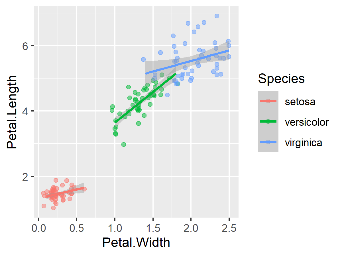
ggplot(data=iris, aes(x = Petal.Width, y = Petal.Length, color = Species)) +
  geom_jitter(alpha = 0.5) +
  geom_smooth(method = "lm")

I want to know the following:

• for each species, is the slope different from zero?
• do slopes differ between species?

I can get some of this information from summary(myModel):

Coefficients:
                              Estimate Std. Error t value Pr(>|t|)    
(Intercept)                     1.3276     0.1309  10.139  < 2e-16 ***
Petal.Width                     0.5465     0.4900   1.115   0.2666    
Speciesversicolor               0.4537     0.3737   1.214   0.2267    
Speciesvirginica                2.9131     0.4060   7.175 3.53e-11 ***
Petal.Width:Speciesversicolor   1.3228     0.5552   2.382   0.0185 *  
Petal.Width:Speciesvirginica    0.1008     0.5248   0.192   0.8480    

In my understanding, this gives:

• the slope for the species "setosa" (Petal.Width)
• the differences in slopes of setosa vs. versicolor (Petal.Width:Speciesversicolor) and setosa vs. virginica (Petal.Width:Speciesvirginica)

I tried to get the other slopes and slope differences through lsmeans::lstrends:

# get slopes
myModelSlopes <- lstrends(myModel, "Species", var="Petal.Width")
myModelSlopes

 Species    Petal.Width.trend    SE  df lower.CL upper.CL
 setosa                 0.546 0.490 144   -0.422     1.52
 versicolor             1.869 0.261 144    1.353     2.39
 virginica              0.647 0.188 144    0.276     1.02

# get differences between slopes
pairs(myModelSlopes)

 contrast               estimate    SE  df t.ratio p.value
 setosa - versicolor      -1.323 0.555 144  -2.382  0.0483
 setosa - virginica       -0.101 0.525 144  -0.192  0.9799
 versicolor - virginica    1.222 0.322 144   3.798  0.0006

From this, I have two questions:

• Is there any way get the p-values for the single slopes (via lsmeans, or another way)? I guess I could always rerun the model using another baseline category, but that seems akward...
• While the estimates seem to be equivalent, I am somewhat confused that pairs(myModelSlopes) gives other p-values for the slope comparisons than summary(myModel). Why is this the case?

Answer 1

I am somewhat confused that pairs(myModelSlopes) gives other p-values for the slope comparisons than summary(myModel). Why is this the case?

Two reasons: they are comparing slightly different things, and they have different handling of multiple comparisons.

Different comparisons

The summary(myModel) is based on tests of whether each coefficient individually is different from 0. That just requires the standard error of each coefficient individually, the square root of its entry on the variance-covariance matrix of the coefficient estimates. Individually, those standard errors are as given in that summary, approximately 0.49, 0.56 and 0.52 for setosa, versicolor, and virginica respectively.

When you compare two different coefficient estimates, you need to take into account both their individual variances and their covariance. See the formula for the variance of a weighted sum of variables. The variance of a difference is the sum of the individual variances minus twice their covariance; you take the square root to get the standard error. As an example, the standard error of the versicolor-virginica difference (items 5 and 6 in the covariance matrix) is:

sqrt(vcov(myModel)[5,5] + vcov(myModel)[6,6] -2*vcov(myModel)[5,6])
# [1] 0.3217766

the value reported by pairs(myModelSlopes).

Multiple comparisons

The standard summary() report of a linear model does no correction for multiple comparisons. In contrast, pairs(myModelSlopes) reports:

# P value adjustment: tukey method for comparing a family of 3 estimates 

Without that adjustment, the two-sided p-value for the versicolor-virginica difference would have been 0.0002:

2*(1-pt(1.222/.322,144))
# [1] 0.000216806

Final note: with respect to your first question, software-specific questions are off-topic here. Check the manual page for summary.emmGrid() to learn about the options, including its infer option. It's generally good to use the most recent version of software; the emmeans package is now preferred to lsmeans.

summary(myModelSlopes,infer=TRUE)
#  Species    Petal.Width.trend    SE  df lower.CL upper.CL t.ratio p.value
#  setosa                 0.546 0.490 144   -0.422     1.52   1.115  0.2666
#  versicolor             1.869 0.261 144    1.353     2.39   7.159  <.0001
#  virginica              0.647 0.188 144    0.276     1.02   3.443  0.0008