Can the jackknife be used to estimate the sample statistic distribution directly a la the bootstrap?
Limiting our discussion to the delete one jackknife, the answer is you "can", but probably shouldn't. It is risky to do so, compared to the bootstrap. Some reasons (this list is not exhaustive) for this include
- The jackknife is limited to $n$ total resamples (compared to $n^n$ for bootstrapping).
- The jackknife resamples are far less robust to outliers.
- In small sample sizes, the behavior of a statistic on $n-1$ data points could be very different from the statistic on $n$ samples. Adjusting via constant multiplication may not fully account for this.
The bootstrap has similar problems, but is far more reliable in most cases.
A case study.
Let's look at the case of inferring the population skewness of an asymmetric distribution.
# Define statistic
sample_skew <- function(xx) mean(((xx-mean(xx))/sd(xx))^3)

# Simulate data
set.seed(12345)
n <- 100 # sample size
x <- rgamma(n, 4.5, 2.5)

# Calculate statistic
theta_hat <- sample_skew(x)
theta_true <- 2/sqrt(4.5) # Gamma theory
Here we get an estimate of $\hat\theta = 0.844$ where the true value is $\theta = 2/\sqrt{4.5} \approx 0.943$. Now we can compare the percentile bootstrap with the percentile and traditional jackknife. Performing a percentile jackknife requires some manipulation.
Tukey proposed studying the psuedo-values
$$\tilde\theta_i = n\hat\theta - (n-1)\hat\theta_{-i}$$
where $\hat\theta_{-i}$ is the estimate we obtain after deleting $x_i$ (the original Tukey paper is hard to find, see this paper for an alternative reference). These values are used to estimate the variance of $\hat\theta$ using the equation:
$$\text{Var}_J(\hat\theta) = \frac{1}{n(n-1)}\sum_{i=1}^n \left(\tilde\theta_i - \frac{1}{n}\sum_{i=1}^n\tilde\theta_i\right)^2$$
and a $(1-\alpha)$ confidence interval is constructed as
$$\hat\theta_{J} \pm z_{\alpha/2} \sqrt{\text{Var}_J(\hat\theta)}$$
where $\hat\theta_J$ is the usual jackknife estimator, i.e. the mean of the $\tilde\theta_i$'s.
This suggests that we can manipulate the pseudo-values to represent samples from the sampling distribution via:
$$\hat\theta_{J,i} = \hat\theta_J + (\tilde\theta_i - \hat\theta_J)n^{-1/2}.$$
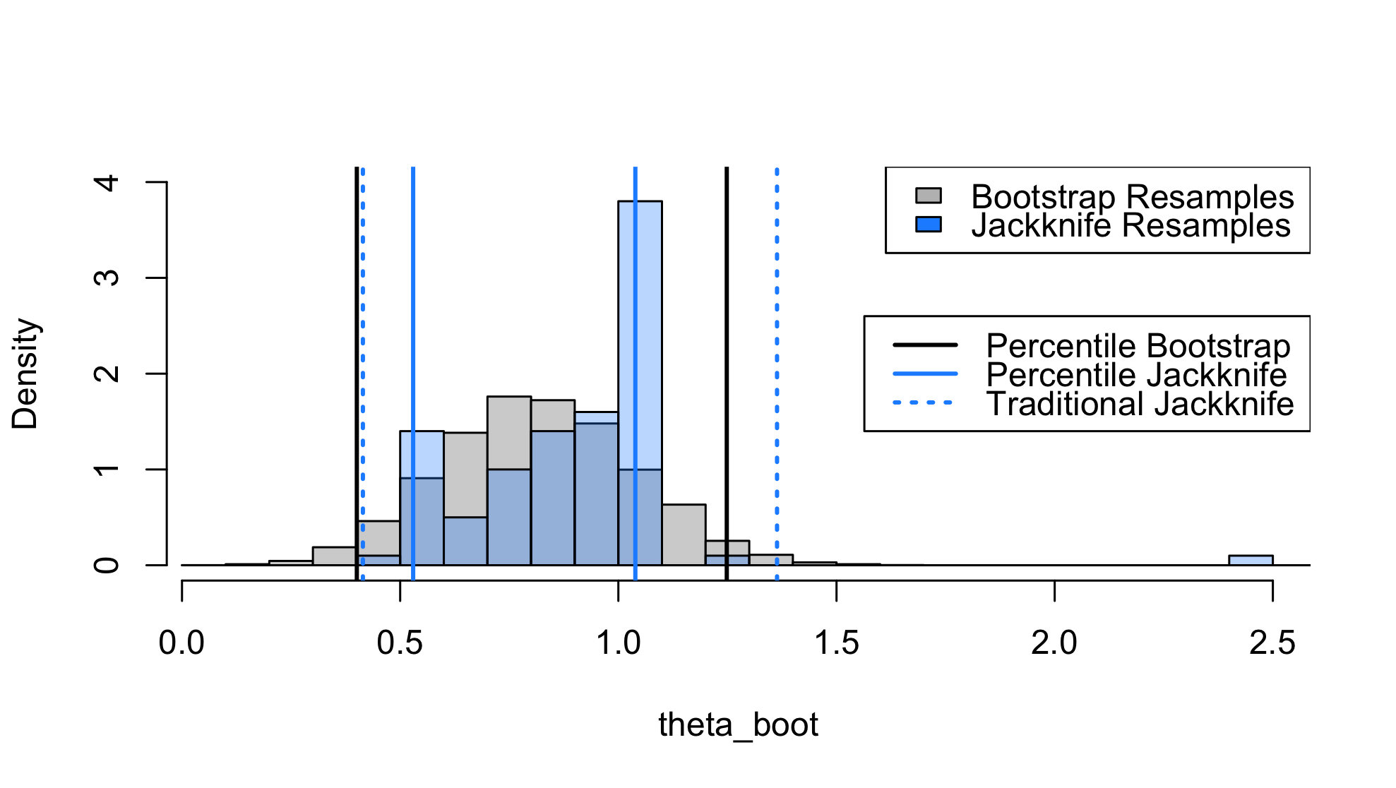
The problem is that (because of the aforementioned warnings) the variance is often driven by extreme outliers, and so the percentile jackknife can be way too anti-conservative. Consider one instance of the problem described above (code given below):

The 95% CI based on jackknife resamples doesn't account for the heavy tails, and is not well-calibrated. In some problems, this might be improved by using a larger sample size and/or using a delete-$d$ jackknife with $d > 1$. But it's still generally inferior to the bootstrap.
Simulation study:
A quick simulation study gives the following results. I will also include results using the accelerated bootstrap, implemented here. These numbers are nominal coverages on $1000$ replications, with a target of $95\%$.
| Sample Size |
Percentile Bootstrap |
Accelerated Bootstrap |
Percentile Jackknife |
Traditional Jackknife |
| n = 10 |
75.3 |
79.9 |
68.0 |
80.4 |
| n = 100 |
80.7 |
84.6 |
68.0 |
85.0 |
| n = 500 |
88.2 |
90.6 |
65.8 |
90.3 |
| n = 1000 |
90.3 |
90.1 |
62.5 |
91.0 |
For this particular problem, the traditional jackknife is quite competitive while the percentile version is flawed. Moreover, increasing the sample size does not seem to help. This is because of the extremely heavy right tail in the distribution of the jackknife resamples.
R Code.
To reproduce the results of the simulation study.
# Set sample size
n <- 100
# Analysis of coverage properties
M <- 1000 # Replications
cov_boot <- cov_boot_a <- cov_jack1 <- cov_jack2 <- 0
for(m in 1:M){
  x <- rgamma(n, 4.5, 2.5)
  theta_hat <- sample_skew(x)

  # Conduct bootstrap
  B <- 2000
  theta_boot <- rep(NA, B)
  for(i in 1:B){
    x_boot <- sample(x, n, replace=TRUE)
    theta_boot[i] <- sample_skew(x_boot)
  }

  # Do Jackknife
  theta_jack <- rep(NA, n)
  for(i in 1:n){
    x_jack <- x[-i]
    theta_jack[i] <- n*theta_hat - (n-1)*sample_skew(x_jack)
  }
  # Do correction on pseudo-values
  theta_jack_samples <- mean(theta_jack) + sqrt(qnorm(1-0.05/2))*(theta_jack - mean(theta_jack))/sqrt(n)

  # Check coverages
  ci_boot <- quantile(theta_boot, c(0.025, 0.975))
  if(ci_boot[1] < theta_true & ci_boot[2] > theta_true){
    cov_boot <- cov_boot + 1/M
  }

  # Accelerated bootstrap github.com/knrumsey/quack
  #ci_boot_a <- quack::boot_accel(x, sample_skew, B=2000, alpha=0.05)
  #if(ci_boot_a[1] < theta_true & ci_boot_a[2] > theta_true){
  #  cov_boot_a <- cov_boot_a + 1/M
  #}

  ci_jack1 <- quantile(theta_jack_samples, c(0.025, 0.975))
  if(ci_jack1[1] < theta_true & ci_jack1[2] > theta_true){
    cov_jack1 <- cov_jack1 + 1/M
  }

  ci_jack2 <- mean(theta_jack) + c(-1, 1)*qnorm(1-0.05/2)*sd(theta_jack)/sqrt(n)
  if(ci_jack2[1] < theta_true & ci_jack2[2] > theta_true){
    cov_jack2 <- cov_jack2 + 1/M
  }
  if((m %% (M/10)) == 0) print(m)
}
And code to recreate the figure for a single replicate.
xx =c(theta_boot, theta_jack_samples)
xxlim = c(floor(min(xx)), ceiling(max(xx)))
hist(theta_boot, freq=FALSE, breaks=seq(xxlim[1], xxlim[2], by=0.1),
     xlim=range(c(theta_boot, theta_jack_samples)), ylim=c(0, 4),
     main="")
hist(theta_jack_samples, add=TRUE, col=adjustcolor("dodgerblue", alpha.f=0.3),
     freq=FALSE, breaks=seq(xxlim[1], xxlim[2], by=0.1))

# 95% confidence intervals
abline(v=quantile(theta_boot, c(0.025, 0.975)), lwd=2)
abline(v=quantile(theta_jack_samples, c(0.025, 0.975)), lwd=2, col='dodgerblue')

abline(v=mean(theta_jack) + c(-1, 1)*qnorm(0.05/2)*sd(theta_jack)/sqrt(n),
       lwd=2, col="dodgerblue", lty=3)

legend("topright", c("Bootstrap Resamples", "Jackknife Resamples"), fill=c('grey', 'dodgerblue'))
legend("right",
       c("Percentile Bootstrap", "Percentile Jackknife", "Traditional Jackknife"),
       col=c("black", "dodgerblue", "dodgerblue"),
       lwd=2, lty=c(1,1,3))
References
Tukey, John. "Bias and confidence in not quite large samples." Ann. Math. Statist. 29 (1958): 614.
Friedl, Herwig, and Erwin Stampfer. "Jackknife resampling." Encyclopedia of environmetrics 2 (2002): 1089-1098.

