Plotting probabilities from multinomial regression output

Question

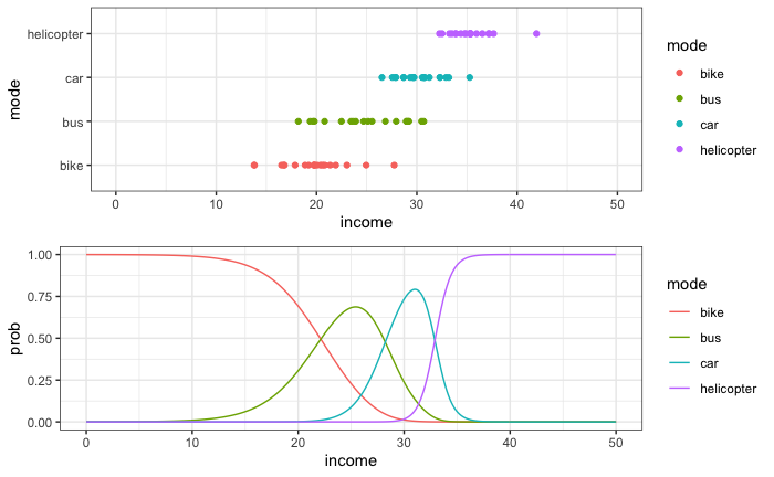
I generated some data to visualize a multinomial logistic regression, where individuals choose a mode of transportation based on their income. I then set up a regression and predicted the probabilities to then plot them. Here's my code:

library(tidyverse)
library(ggpubr)
library(nnet)

# Generating the data --------------------------
set.seed(100)
helicopter <- rnorm(20, mean = 35, sd = 3)
car <- rnorm(20, mean = 30, sd = 3)
bus <- rnorm(20, mean = 25, sd = 3)
bike <- rnorm(20, mean = 20, sd = 3)

transportation_data <- data.frame(helicopter, car, bus, bike) %>%
  pivot_longer(cols = 1:4, values_to = "income", names_to = "mode")

# Plotting the data ---------------------------
transportation_plot <- transportation_data %>%
  ggplot(aes(x = income, y = mode, color = mode))+
  geom_point()+
  coord_cartesian(xlim = c(0,50))

# Setting up the regression -------------------
transportation_regression <- multinom(mode~income, data = transportation_data)
summary(transportation_regression)

# Predicting the probabilities ---------------
new_data <- data.frame(income = seq(0,50,0.1))
prediction <- as.data.frame(predict(transportation_regression, new_data, type = "probs"))
new_data <- cbind(new_data, prediction)

# Plotting the probabilities -----------------
prob_plot <- new_data %>%
  pivot_longer(2:5, names_to = "mode", values_to = "prob") %>%
  ggplot(aes(x = income, y = prob, color = mode))+
  geom_line()

# Merging the two plots -----------------------
ggarrange(transportation_plot, prob_plot, nrow = 2)

The regression output is:

Coefficients:
           (Intercept)    income
bus          -8.458078 0.3821646
car         -26.317817 1.0150949
helicopter  -69.080279 2.3148401

And the plot looks like this:

What I would like to do now is to plot the same probabilities, but not using the predict() function. I want to use stat_function() and the coefficients of the regression output. My uni-script says that the probability of the choice of alternative j is $Pr(y_i = j | \bf{x_i}) = \frac{exp(\bf{x_i\prime \beta_j})}{\sum_{h=1}^J exp(\bf{x_i\prime \beta_h})}$ so I guess I need this function. But I have trouble understanding and implementing this.

EDIT

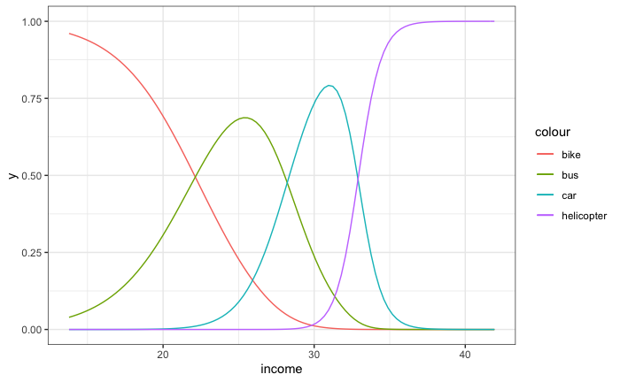
I tried the following, but it does not yield reasonable results:

ins <- coef(transportation_regression)[1:3]
betas <- coef(transportation_regression)[4:6]

transportation_data %>%
  ggplot(aes(x = income))+
  stat_function(fun = function(x) { exp(1) / (1 + sum(exp(ins + betas * x))) }, aes(color = "bike"))+
  stat_function(fun = function(x) { exp(ins[1] + betas[1] * x) / (1 + sum(exp(ins + betas * x))) }, aes(color = "bus"))+
  stat_function(fun = function(x) { exp(ins[2] + betas[2] * x) / (1 + sum(exp(ins + betas * x))) }, aes(color = "car"))+
  stat_function(fun = function(x) { exp(ins[3] + betas[3] * x) / (1 + sum(exp(ins + betas * x))) }, aes(color = "helicopter"))

However, if I take one of the function, let's say for car and plug in 30 for x in the console, I get a sensible result (compare to the plot above):

> exp(ins[2] + betas[2] * 30) / (1 + sum(exp(ins + betas * 30)))
[1] 0.73385

So why won't it work as a function of x in ggplot?

Answer 1

As COOLSerdash suggested, swapping 1 + sum(exp(ins + betas * x)) with
1 + sapply(x, \(x){sum(exp(ins + betas * x))}) worked:

transportation_data %>%
  ggplot(aes(x = income))+
  stat_function(fun = function(x) { 1 / (1 + sapply(x, \(x){sum(exp(ins + betas * x))})) }, aes(color = "bike"))+
  stat_function(fun = function(x) { exp(ins[1] + betas[1] * x) / (1 + sapply(x, \(x){sum(exp(ins + betas * x))})) }, aes(color = "bus"))+
  stat_function(fun = function(x) { exp(ins[2] + betas[2] * x) / (1 + sapply(x, \(x){sum(exp(ins + betas * x))})) }, aes(color = "car"))+
  stat_function(fun = function(x) { exp(ins[3] + betas[3] * x) / (1 + sapply(x, \(x){sum(exp(ins + betas * x))})) }, aes(color = "helicopter"))