Probability of a given result with multiples of mixed dice with different number of faces

Question

What is the formula to calculate the probability of getting 41 when I throw two 10-sided dice and four 8-sided dice? I’m looking for an algorithm for the general case of throwing multiples of two sets of differently-faced dice.

Code if same number of faces

Here is some Typescript based on the Python code here that gives the probability if all the dice have the same number of faces:

function probabilityOfN(dice: number, sides: number, n: number): number {
    return Array.from({length: sides}, (_, i) => (1 / sides) * probabilityOfN(dice - 1, sides, n - i - 1))
        .reduce((a, b) => a + b)
}

Missing code if different number of faces

function probabilityOfN(diceA: number, sidesA: number, diceB: number, sidesB: number, n: number): number {
    // ???
}

The question is how to do the calculation for this function? Could be in Python as well.

Test case

Given:

• diceA = 2
• sidesA = 10
• diceB = 4
• sidesB = 8
• n = 41

Then according to https://dice.clockworkmod.com/ the probability should come out as 0.01

Answer 1

The brute force method would be to order your dice, enumerate all possible combinations of throws, count the number of "successful" throws and divide by the total number of possible throws. In your particular case, you have $10^2\times 8^4=409,600$ possible throws. A few lines of code tell you that $4,132$ of these show a total of 41. So the probability is indeed $\frac{4,132}{409,600}\approx 0.01$.

In R (sorry, I'm more fluent in R, but this should be understandable):

dice <- c(rep(10,2),rep(8,4))
all_possible_combos <- expand.grid(sapply(dice,function(n)1:n))
sum(rowSums(all_possible_combos)==41)
nrow(all_possible_combos)

The key part is the expand.grid() function that gives you all possible combinations. Here is the analogous histogram to yours:

hist(rowSums(all_possible_combos),breaks=seq(-0.5,sum(dice)+0.5))

This works quickly enough with just six dice, and does not rely on the fact that you have only two types of dice. If you have much more, you may run into a combinatorial explosion. In this case, it may make sense to treat each group separately (see How to easily determine the results distribution for multiple dice?) and sum over the possible ways to split the target number of 41 between the two groups of dice. The question just is whether the gain in performance outweighs the loss in understandability.

Answer 2

I would suggest using a generating polynomial to do this. The idea is to represent the contribution of one die towards the total by the power series $(x^1 + x^2 + \dots + x^n)$ where $n$ is the number of faces on the die, then multiplying together one series per die and calculating the coefficient of the power of the sum you're looking for, e.g., the coefficient of $x^{41}$ in your example. Then you can divide by the number of different possible die rolls to get the result as a probability.

This works because expanding all the terms in the product is analogous to listing all the possible combinations of die rolls on your dice, e.g., rolling a 1 on all 6 dice in the question is represented by choosing the $x^1$ term from the series for each die and multiplying these together to get $x^6$. So with the 6 dice in the question, there is only 1 way to roll a total of 6. Similarly, there will be many different rolls that give a sum of 41 and number of these will be equal to the coefficient of $x^{41}$.

You can reduce the degree of combinatorial explosion by discarding terms where the power of $x$ exceeds the target, or cannot reach it based on the remaining terms in the product.

Wolfram Alpha pseudocode:

Coefficient(sum(x^n, n=1 to 10)^2 * sum(x^n, n=1 to 8)^4, x^41) / (10^2 * 8^4)

Sample calculation

Answer 3

Using @Henry's suggestion of recursion over the dice, below is an R function that will return the full PMF of the sum resulting from rolling a set of fair dice with number of faces of each die given by the vector d.

The function manages combinatorial explosion by summing the probability by each possible cumulative die roll at each iteration. So the length of the PMF after iteration $i$ is:

$$1-i+\sum_{j=1}^id_j$$

I also provide a function employing the fast Fourier transform.

---

Recursive Algorithm

To illustrate the recursive algorithm, consider rolling three 4-sided dice. Initialize the result by starting with the first die roll.

d <- rep(4, 3) # 3d4
v <- 1:d[1] # initialize the total value of the rolls
p <- rep(1/d[1], d[1]) # the probability of each value

Calculate all possible results of adding the first roll to the second roll and their probabilities.

(mv <- outer(v, 1:d[2], "+"))
#>      [,1] [,2] [,3] [,4]
#> [1,]    2    3    4    5
#> [2,]    3    4    5    6
#> [3,]    4    5    6    7
#> [4,]    5    6    7    8
(mp <- outer(p, rep(1/d[2], d[2])))
#>        [,1]   [,2]   [,3]   [,4]
#> [1,] 0.0625 0.0625 0.0625 0.0625
#> [2,] 0.0625 0.0625 0.0625 0.0625
#> [3,] 0.0625 0.0625 0.0625 0.0625
#> [4,] 0.0625 0.0625 0.0625 0.0625

Aggregate probabilities by value to get the PMF of the first two rolls.

(p <- sapply(split(mp, mv), sum))
#>      2      3      4      5      6      7      8 
#> 0.0625 0.1250 0.1875 0.2500 0.1875 0.1250 0.0625
(v <- as.integer(names(p)))
#> [1] 2 3 4 5 6 7 8

Repeat the process by adding the result of the third roll to the first two.

(mv <- outer(v, 1:d[3], "+"))
#>      [,1] [,2] [,3] [,4]
#> [1,]    3    4    5    6
#> [2,]    4    5    6    7
#> [3,]    5    6    7    8
#> [4,]    6    7    8    9
#> [5,]    7    8    9   10
#> [6,]    8    9   10   11
#> [7,]    9   10   11   12
(mp <- outer(p, rep(1/d[3], d[3])))
#>       [,1]     [,2]     [,3]     [,4]
#> 2 0.015625 0.015625 0.015625 0.015625
#> 3 0.031250 0.031250 0.031250 0.031250
#> 4 0.046875 0.046875 0.046875 0.046875
#> 5 0.062500 0.062500 0.062500 0.062500
#> 6 0.046875 0.046875 0.046875 0.046875
#> 7 0.031250 0.031250 0.031250 0.031250
#> 8 0.015625 0.015625 0.015625 0.015625
(p <- sapply(split(mp, mv), sum))
#>        3        4        5        6        7        8        9       10 
#> 0.015625 0.046875 0.093750 0.156250 0.187500 0.187500 0.156250 0.093750 
#>       11       12 
#> 0.046875 0.015625
(v <- as.integer(names(p)))
#>  [1]  3  4  5  6  7  8  9 10 11 12

Notice that the probability matrix is constant across each row, so we can use cumsum instead of outer to speed up the algorithm. We can also wait until the end to generate the vector v.

droll <- function(d) {
  d <- sort(d, TRUE)
  p <- rep(1/d[1], d[1])
  
  if (length(d) > 1L) {
    for (x in d[-1]) {
      cs <- cumsum(p/x)
      k <- length(p) - x
      p <- c(
        cs[1:x],
        cs[seq.int(x + 1, length.out = k)] - cs[seq_len(k)],
        cs[length(p)] - cs[(k + 1):(length(p) - 1)]
      )
    }
  }
  
  list(v = length(d):sum(d), p = p)
}

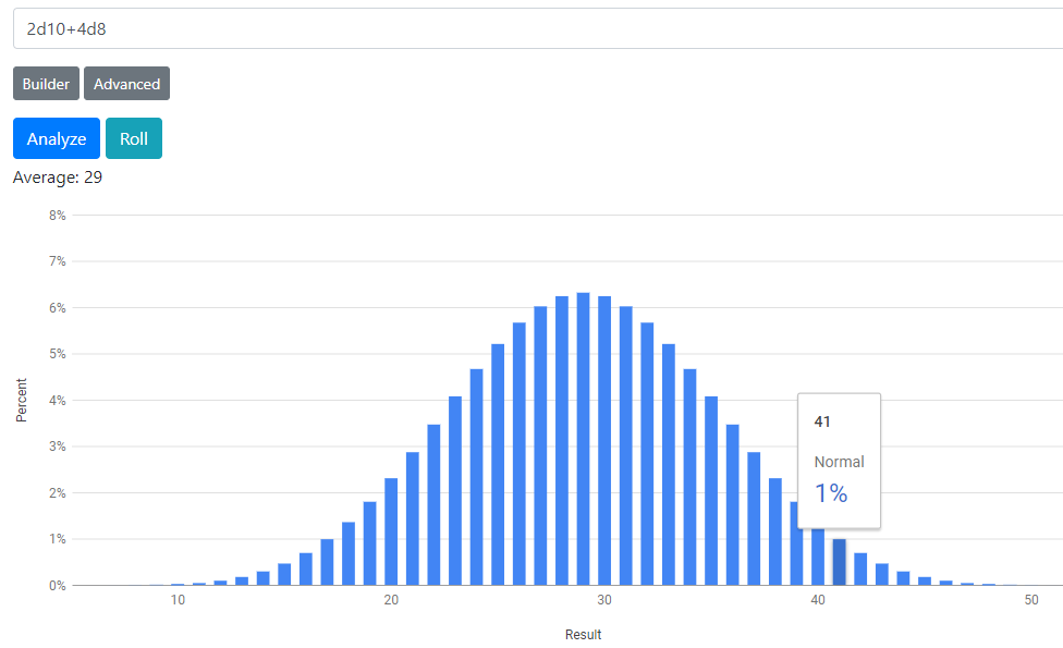
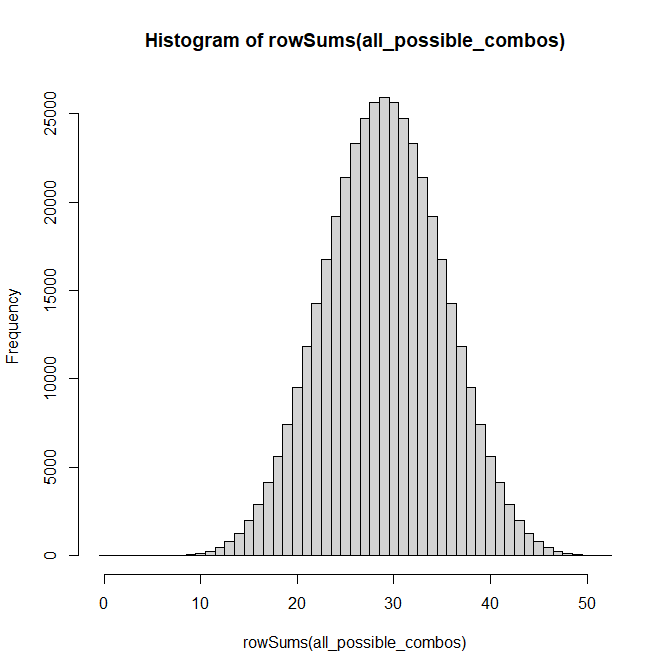
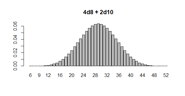
Testing with four 8-sided and two 10-sided dice:

# 4d8 + 2d10
with(
  droll(rep.int(c(8, 10), c(4, 2))),
  barplot(p, names.arg = v, main = "4d8 + 2d10")
)

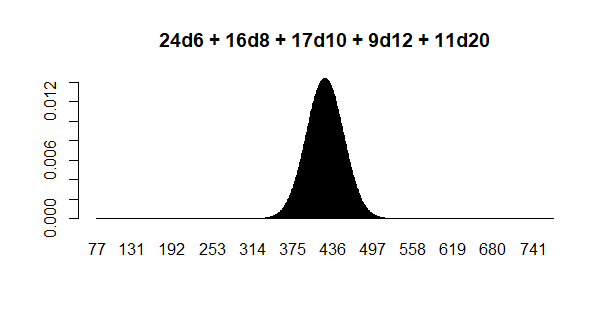
A larger test:

# 24d6 + 16d8 + 17d10 + 9d12 + 11d20
with(
  droll(rep.int(c(6, 8, 10, 12, 20), c(24, 16, 17, 9, 11))),
  barplot(p, names.arg = v, main = "24d6 + 16d8 + 17d10 + 9d12 + 11d20")
)

---

Fast Fourier Transform

If many of the dice share the same number of sides, the fast Fourier transform is more performant still, requiring a single transform for each denomination of dice and one inverse transform.

droll.fft <- function(d) {
  n <- table(d)
  d <- as.integer(names(n))
  maxroll <- sum(n*d)
  r <- maxroll - sum(n) + 1
  N <- as.integer(2^ceiling(log2(r)))
  p <- fft(rep.int(c(1/d[1], 0), c(d[1], N - d[1])))^n[1]
  
  if (length(d) > 1L) {
    for (i in 2:length(d)) {
      p <- p*fft(rep.int(c(1/d[i], 0), c(d[i], N - d[i])))^n[i]
    }
  }
  
  list(v = sum(n):maxroll, p = Re(fft(p, TRUE)[1:r])/N)
}

microbenchmark::microbenchmark(
  droll = droll(rep.int(c(6, 8, 10, 12, 20), c(24, 16, 17, 9, 11))),
  droll.fft = droll.fft(rep.int(c(6, 8, 10, 12, 20), c(24, 16, 17, 9, 11))),
  check = "equal"
)
#> Unit: microseconds
#>       expr   min     lq     mean median      uq    max neval
#>      droll 658.6 853.90 1201.909 949.20 1039.35 9536.1   100
#>  droll.fft 306.6 332.45  356.929 346.85  372.40  576.2   100

Answer 4

Based on @Stephan’s beautiful answer, here is the Typescript code for posterity:

function probabilityOfNwithDifferentFaces(n: number, ...allDiceAndSides: [number, number][]): number {
    if (!allDiceAndSides.length) return 0
    // trying to avoid combinatorial explosion
    const cleaned = allDiceAndSides.filter(([dice, sides]) => dice > 0 && sides > 0 && dice < 100 && sides <= 100)
        .slice(0, 7)
    if (cleaned.length === 1) return probabilityOfN(cleaned[0][0], cleaned[0][1], n)
    const minResult = cleaned.reduce((acc, [dice]) => acc + dice, 0)
    const maxResult = cleaned.reduce((acc, [dice, sides]) => acc + dice * sides, 0)
    if (n < minResult || n > maxResult) return 0
    cleaned.sort((a, b) => b[1] - a[1])
    const allRepeats: number[] = cleaned.flatMap(([dice, sides]) => Array(dice).fill(sides))
    // console.log(allRepeats)
    const all_possible_combos: number[][] = []
    for (let i = 1; i <= allRepeats.length; i++) {
        const die_combos: number[] = []
        for (let j = 1; j <= allRepeats[i - 1]; j++) {
            die_combos.push(j)
        }
        all_possible_combos.push(die_combos)
    }
    const cartesian_product = (...arrays: any[]) => arrays.reduce(
        (a, b) => a.flatMap((d: any) => b.map((e: any) => [d, e].flat())))
    const all_combinations = cartesian_product(...all_possible_combos)
    // @ts-ignore
    const sum_of_rows = all_combinations.map(row => row.reduce((a, b) => a + b))
    // @ts-ignore
    const count_of_rows_summing_to_n = sum_of_rows.filter(sum => sum === n).length
    // console.log(count_of_rows_summing_to_n)
    const totalPossibleThrows = all_combinations.length
    // console.log(totalPossibleThrows)
    // console.log(probability)
    return count_of_rows_summing_to_n / totalPossibleThrows
}

And some use cases:

function calculateAndReportWithDifferentFaces(n: number, ...allDiceAndSides: [number, number][]) {
    const p = probabilityOfNwithDifferentFaces(n, ...allDiceAndSides)
    const rollString = allDiceAndSides.map(([dice, sides]) => `${dice}d${sides}`).join(" + ")
    console.log(`Got ${p.toFixed(3)} for ${n} with ${rollString}`)
}

function differentFacesProbabilityTest() {
    console.log("=== Individual probabilities with different faces")
    calculateAndReportWithDifferentFaces(2, [1, 10], [1, 6])
    calculateAndReportWithDifferentFaces(9, [1, 10], [1, 6])
    calculateAndReportWithDifferentFaces(14, [1, 10], [1, 6])
    calculateAndReportWithDifferentFaces(15, [1, 10], [1, 6])
    calculateAndReportWithDifferentFaces(16, [1, 10], [1, 6])
    calculateAndReportWithDifferentFaces(31, [2, 10], [4, 8])
    calculateAndReportWithDifferentFaces(41, [2, 10], [4, 8])
    calculateAndReportWithDifferentFaces(41, [4, 8], [2, 10])
    console.log("Same faces check:")
    calculateAndReportWithDifferentFaces(2, [2, 10])
    calculateAndReportWithDifferentFaces(11, [2, 10])
    calculateAndReportWithDifferentFaces(19, [2, 10])
    calculateAndReportWithDifferentFaces(20, [2, 10])
    console.log("Incorrect inputs:")
    calculateAndReportWithDifferentFaces(5, [2, 10], [4, 8])
    calculateAndReportWithDifferentFaces(53, [2, 10], [4, 8])
}