Understanding emmeans outputs for poisson and negative binomial GLM fitted on count data with or without offset

Question

I fitted a poisson and negative binomial GLM on count data (=larva) and try to explain it as a function of a factor (=modality). However, as the traps used to trap larvae from inflorescences were exposed to different number of inflorescences, I than added an offset (=inflo) to the models for count normalization (in this case I am modeling the number of larvae per inflorescence).

I used the following data:

mydata <- data.frame(
 modality = c("ER","ER","ER","ER","ER","ER","ER","ER","ER","ER","ER","ER","ER","ER","EH","EH","EH","EH","EH","EH","EH","EH","EH","EH","EH","EH","EH","EH","EH","EH","EH","EH","TS","TS","TS","TS","TS","TS","TS","TS","TS","TS","TS","TS","TS","TS"),
 larva = c(149,184,51,35,10,6,102,29,151,37,57,95,44,38,2,245,29,22,30,32,124,42,17,49,39,36,60,14,73,22,16,21,21,54,53,39,41,58,47,42,12,1,4,2,3,1),
 inflo = c(61,48,68,28,33,15,49,31,87,40,21,27,25,20,9,10,28,23,20,32,102,34,18,31,33,32,86,17,77,58,20,22,50,53,38,31,21,35,78,48,15,22,3,10,13,5)
  ) %>%
 mutate(rate = larva / inflo)

Mean values per modality for count and rate data are :

mydata_stat <- mydata %>%
 group_by(modality) %>%
 summarise(mean_larva = mean(larva),
           mean_inflo = mean(inflo),
           mean_rate = mean(rate),
           n = length(larva)
 )
mydata_stat

# A tibble: 3 x 5
  modality mean_larva mean_inflo mean_rate     n
  <chr>         <dbl>      <dbl>     <dbl> <int>
1 EH             48.5       36.2     2.28     18
2 ER             70.6       39.5     1.75     14
3 TS             27         30.1     0.856    14

From what I understand, a count GLM models the conditional mean of counts. If μ is the mean response conditional on the level of modality and the log-link function is η = log(μ), then the model is:
η = β0 + β1 modalityER + β2 modalityTS, that is:
μ = exp(β0 + β1 modalityER + β2 modalityTS)
And for count GLM with an offset models the conditional mean of normalized counts. In this case, the model is:
η = β0 + β1 modalityER + β2 modalityTS + log(inflo), that is:
μ / inflo = exp(β0 + β1 modalityER + β2 modalityTS)

1/ Here the models and emmeans outputs for the Poisson and negative binomial GLMs without offset:

fit1 <- glm(larva ~ modality, family = "poisson", data = mydata)
emmeans(fit1, ~ modality, type="response")

 modality rate   SE  df asymp.LCL asymp.UCL
 EH       48.5 1.64 Inf      45.4      51.8
 ER       70.6 2.25 Inf      66.3      75.1
 TS       27.0 1.39 Inf      24.4      29.9

Confidence level used: 0.95 
Intervals are back-transformed from the log scale

fit3 <- glm.nb(larva ~ modality, data = mydata)
emmeans(fit3, ~ modality, type="response")

 modality response    SE  df asymp.LCL asymp.UCL
 EH           48.5 10.59 Inf      31.6      74.4
 ER           70.6 17.40 Inf      43.5     114.4
 TS           27.0  6.75 Inf      16.5      44.1

Confidence level used: 0.95 
Intervals are back-transformed from the log scale 

I was expecting that the response means provided by emmeans was equal to observed means (=mean_larva in mydata_stat), which is the case for both models.

2/ Here the models and emmeans outputs for the Poisson and negative binomial GLMs with offset:

fit1_offset <- glm(larva ~ modality + offset(log(inflo)), family = "poisson", data = mydata)
emmeans(fit1_offset, ~ modality, type="response", offset = log(1))

 modality  rate     SE  df asymp.LCL asymp.UCL
 EH       1.339 0.0453 Inf      1.25     1.431
 ER       1.787 0.0568 Inf      1.68     1.902
 TS       0.896 0.0461 Inf      0.81     0.991

fit3_offset <- glm.nb(larva ~ modality + offset(log(inflo)), data = mydata)
emmeans(fit3_offset, ~ modality, type="response", offset = log(1))

 modality response    SE  df asymp.LCL asymp.UCL
 EH          2.245 0.478 Inf     1.478      3.41
 ER          1.755 0.424 Inf     1.093      2.82
 TS          0.861 0.215 Inf     0.528      1.41

Confidence level used: 0.95 
Intervals are back-transformed from the log scale

In the case of count GLMs with offset, I was also expecting that the response rates provided by emmeans was equal to observed rates (=mean_rate in mydata_stat), which is not the case.
In the case of the negative binomial GLM, it was close to mean_rate but not exactly the same, particularly for EH modality. And in the case of the Poisson GLM, it was instead exactly equal to mean_rate_2 = mean_larva / mean_inflo.

mydata_stat %>% mutate(mean_rate_2 = mean_larva / mean_inflo)

# A tibble: 3 x 6
  modality mean_larva mean_inflo mean_rate     n mean_rate_2
  <chr>         <dbl>      <dbl>     <dbl> <int>       <dbl>
1 EH             48.5       36.2     2.28     18       1.34 
2 ER             70.6       39.5     1.75     14       1.79 
3 TS             27         30.1     0.856    14       0.896

I can't understand why...

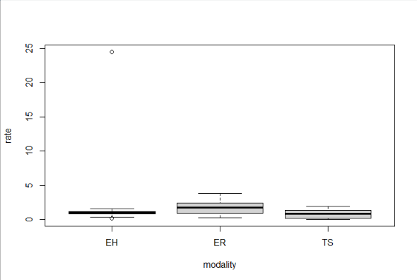
I realized that there is a possible oulier in modality EH:

boxplot(rate ~ modality, data=mydata)

When removing the outlier, response rates provided by emmeans were much more closer between the two models and also closer the observed rates (=mean_rate in mydata_stat_cor - see below) :

mydata_cor <- mydata %>% filter(rate < 20)
mydata_stat_cor <- mydata_cor %>%
 group_by(modality) %>%
 summarise(mean_larva = mean(larva),
           mean_inflo = mean(inflo),
           mean_rate = mean(rate),
           n = length(larva)
 )
mydata_stat_cor %>% mutate(mean_rate_2 = mean_larva / mean_inflo)

# A tibble: 3 x 6
  modality mean_larva mean_inflo mean_rate     n mean_rate_2
  <chr>         <dbl>      <dbl>     <dbl> <int>       <dbl>
1 EH             36.9       37.8     0.976    17       0.978
2 ER             70.6       39.5     1.75     14       1.79 
3 TS             27         30.1     0.856    14       0.896

fit1_offset <- glm(larva ~ modality + offset(log(inflo)), family = "poisson", data = mydata_cor)
fit3_offset <- glm.nb(larva ~ modality + offset(log(inflo)), data = mydata_cor)

as.data.frame(emmeans(fit1_offset, ~ modality, type="response", offset = log(1)))$rate
[1] 0.9781931 1.7866184 0.8957346

as.data.frame(emmeans(fit3_offset, ~ modality, type="response", offset = log(1)))$response
[1] 0.9833245 1.7576010 0.8702802

Does it mans that mean_rates are managed differently in Poisson and Negative binomila GLMs? How can these differences in results be explained ? Thanks in advance for your helpful explanations.

Answer 1

First of all, the one question I actually can answer is the one about dividing by the mean inflo. This is indeed the case; look at:

> emmeans(fit3_offset, "modality")@grid
  modality .offset. .wgt.
1       EH 3.565852    18
2       ER 3.565852    14
3       TS 3.565852    14

> log(mean(mydata$inflo))
[1] 3.565852

This happens because inflo is considered a covariate in the model, and emmeans() by default sets covariates to their mean, making the offset equal to the log of that mean.. If we do not specify offset in the emmeans() call, then we are adding the .offset. to the linear estimates. If on the other hand we specify offset = 0, then all the estimates will be smaller by that amount; so on the response scale, we'll get the estimates divided by the mean inflo.

I think what is happening here is that, while we indeed have a model for the mean rates (inasmuch that the log offsets are subtracted from the log responses, log(larva) - log(inflo) = log(larva/inflo)), the estimates are just not the same mean rates you computed; it's more complicated than that. If we go back to the the model predictions and compute the rates from those, we can reproduce the estimated rates obtained from emmeans():

> tapply(exp(predict(fit1_offset)) / mydata$inflo, mydata$modality, mean)
       EH        ER        TS 
1.3389571 1.7866184 0.8957346 

> tapply(exp(predict(fit3_offset)) / mydata$inflo, mydata$modality, mean)
       EH        ER        TS 
2.2445143 1.7552025 0.8613856 

Both of these are legitimate estimates of mean rates; they are just different models so they yield different results.

Answer 2

TLDR: I don't address the question how emmeans handles an offset in a count model, which is answered by @RussLenth (+1). Instead I plot the data which suggests that the counts are overdispersed, with a different dispersion in each modality.

Let's start by plotting the data. We can do better than a boxplot by showing larva against inflo by modality.

We learn lots from these three scatterplots:

• There is a linear relationship between inflo and larva, so the model should include inflo as an offset. (You have already done this.)
• The counts are overdispersed, esp. for the ER modality. A Poisson model won't be appropriate for this data; instead consider a quasipoisson model or a negative binomial model.
• The dispersion (ie. the variance) is different for the different modalities. For example, even by eye, ER has about twice as much variability than EH.
• There is an outlier in the EH subset. You should check whether this might be a data entry issue.
• But even more intriguingly, there seems to be a shift in the rate above inflo = 50 or so. If we ignore the outlier, notice how a straight line that fits the points below inflo = 50 will pass above the observations for inflo = 50. Something might have happened during the experiment or else there might be something that happenes to larva when the inflo is too high? There are few observations collected at high inflo, so the data can't tell what's going on.

So to summarize: The data suggests to consider a quasipoisson or a negative binomial model and model the dispersion as well as the mean rate as a function of modality. Since modality is a factor variable, I make a first stab at this analysis by fitting three separate models, one for each modality. I fit both the quasipoisson and the negative binomial regression; the results are similar.

Note: I remove the outlier before I do the analysis.

Here are the estimated dispersion parameters from the quasipoisson models of each modality. These are substantially different and indicate that it may not be reasonable to assume the same dispersion across modalities (as fit1 and fit3 do implicitly).

#>   modality dispersion
#> 1 EH             3.88
#> 2 ER            24.4 
#> 3 TS             9.08

Estimates of the rate $\mu$ with quasipoisson regression:

#>   modality estimate conf.low conf.high
#> 1 EH          0.978    0.835      1.14
#> 2 ER          1.79     1.29       2.39
#> 3 TS          0.896    0.650      1.20

as well as with negative binomial regression:

#>   modality estimate conf.low conf.high
#> 1 EH          0.989    0.842      1.17
#> 2 ER          1.76     1.28       2.51
#> 3 TS          0.864    0.589      1.32

Notice that — should we assume to trust the confidence intervals produced by the two analyses — the CI for the ER rate doesn't overlap with the CIs for the EH and TS rates.

And finally, the data (with one "unusual" data point removed) and with the mean rate estimated by the quasipoisson regression. The model for the EH modality is not a great fit: notice how the line does its best to fit the observations for low inflo (< 50) and high inflo (> 50) with the end result that it fits neither particularly convincingly.

---

R code to reproduce the analysis and the figures:

library("MASS")
library("broom")
library("tidyverse")

calculate_dispersion <- function(object) {
  # NOTE: This snippet is copied from `summary.glm`.
  df.r <- object$df.residual
  fam <- object$family
  if (!is.null(fam$dispersion) && !is.na(fam$dispersion)) {
    fam$dispersion
  } else if (fam$family %in% c("poisson", "binomial")) {
    1
  } else if (df.r > 0) {
    est.disp <- TRUE
    if (any(object$weights == 0)) {
  warning("observations with zero weight not used for calculating dispersion")
}
sum((object$weights * object$residuals^2)[object$weights > 0]) / df.r
  } else {
    est.disp <- TRUE
    NaN
  }
}

mydata <-
  tibble(
    modality = c("ER", "ER", "ER", "ER", "ER", "ER", "ER", "ER", "ER", "ER", "ER", "ER", "ER", "ER", "EH", "EH", "EH", "EH", "EH", "EH", "EH", "EH", "EH", "EH", "EH", "EH", "EH", "EH", "EH", "EH", "EH", "EH", "TS", "TS", "TS", "TS", "TS", "TS", "TS", "TS", "TS", "TS", "TS", "TS", "TS", "TS"),
    larva = c(149, 184, 51, 35, 10, 6, 102, 29, 151, 37, 57, 95, 44, 38, 2, 245, 29, 22, 30, 32, 124, 42, 17, 49, 39, 36, 60, 14, 73, 22, 16, 21, 21, 54, 53, 39, 41, 58, 47, 42, 12, 1, 4, 2, 3, 1),
    inflo = c(61, 48, 68, 28, 33, 15, 49, 31, 87, 40, 21, 27, 25, 20, 9, 10, 28, 23, 20, 32, 102, 34, 18, 31, 33, 32, 86, 17, 77, 58, 20, 22, 50, 53, 38, 31, 21, 35, 78, 48, 15, 22, 3, 10, 13, 5)
  ) %>%
  arrange(
    modality
  )

mydata %>%
  ggplot(
    aes(inflo, larva)
  ) +
  geom_point() +
  facet_grid(
    ~modality
  )

# Remove 1 outlier.
mydata <- mydata %>%
  filter(
    larva < 200
  )

fits <- mydata %>%
  group_by(
    modality
  ) %>%
  nest(
    data = c(larva, inflo)
  ) %>%
  mutate(
    fit.qp = map(data, ~ glm(larva ~ 1 + offset(log(inflo)), family = quasipoisson, data = .)),
    fit.nb = map(data, ~ glm.nb(larva ~ 1 + offset(log(inflo)), data = .))
  )

fits %>%
  mutate(
    dispersion = map_dbl(fit.qp, ~ calculate_dispersion(.))
  ) %>%
  select(
    modality, dispersion
  )

mus.qp <- fits %>%
  mutate(
    tidy = map(fit.qp, tidy, conf.int = TRUE, exponentiate = TRUE)
  ) %>%
  unnest(
    tidy
  ) %>%
  select(
    modality, estimate, conf.low, conf.high
  )
mus.qp

mus.nb <- fits %>%
  mutate(
    tidy = map(fit.nb, tidy, conf.int = TRUE, exponentiate = TRUE)
  ) %>%
  unnest(
    tidy
  ) %>%
  select(
    modality, estimate, conf.low, conf.high
  )
mus.nb

mydata %>%
  ggplot(
    aes(inflo, larva)
  ) +
  geom_point() +
  facet_grid(
    ~modality
  ) +
  geom_abline(
    aes(intercept = 0, slope = estimate, group = modality),
    data = mus.qp
  )