Computation of polynomial contrast variables

Question

Please give me idea how to efficiently recode a categorical variable (factor) into the set of orthogonal polynomial contrast variables.

For many types of contrast variables (e.g. deviation, simple, Helmert, etc.) the pass is:

1. Compose the contrast coefficients matrix correspondig to the type.
2. Inverse or generalize-inverse it to obtain the matrix of codes.

For example:

Suppose there is 3-group factor and we want to recode it into a set of deviation  contrast variables.
The last group is treated as reference. Then the contrast coefficients matrix L is

         Group1 Group2 Group3
   var1   2/3   -1/3   -1/3
   var2  -1/3    2/3   -1/3

and ginv(L) is then the sought-for coding matrix

         var1 var2
  Group1   1    0
  Group2   0    1
  Group3  -1   -1

(We might also use inv(L) instead if we add a row for constant, equal to 1/3, at the head of L.)

Is there the same or similar way to get polynomial contrast variables? If yes what matrix C would look like and how to compose it? If no what still is the way to compute the polynomial contrast variables efficiently (e.g. by matrix algebra).

Answer 1

As a segue to my prior post on this topic I want to share some tentative (albeit incomplete) exploration of the functions behind the linear algebra and related R functions. This is supposed to be a work in progress.

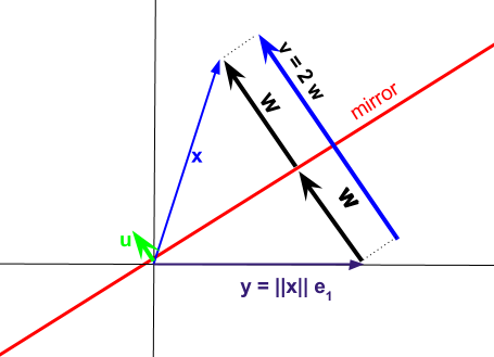
Part of the opaqueness of the functions has to do with the "compact" form of the Householder $\mathbf {QR}$ decomposition. The idea behind the Householder decomposition is to reflect vectors across a hyperplane determined by a unit-vector $\mathbf u$ as in the diagram below, but picking this plane in a purposeful way so as to project every column vector of the original matrix $\bf A$ onto the $\bf e_1$ standard unit vector. The normalized norm-2 $1$ vector $\bf u$ can be used to compute the different Householder transformations $\mathbf{ I - 2\, uu^T x}$.

The resultant projection can be expressed as

$\text{sign}(x_i=x_1)\times \lVert x \rVert \begin{bmatrix}1\\0\\0\\\vdots\\0\end{bmatrix}+\begin{bmatrix}x_1\\x_2\\x_3\\\vdots\\x_m\end{bmatrix}$

The vector $\bf v$ represents the difference between the column vectors $\bf x$ in the matrix $\bf A$ that we want to decompose and the vectors $\bf y$ corresponding to the reflection across the subspace or "mirror" determined by $\bf u$.

The method used by LAPACK liberates the need for storage of the first entry in the Householder reflectors by turning them into $1$'s. Instead of normalizing the vector $\bf v$ to $\bf u$ with $\lVert u\rVert= 1$, it is just the fist entry that is converted to a $1$; yet, these new vectors - call them $\bf w$ can still be used as a directional vectors.

The beauty of the method is that given that $\bf R$ in a $\bf QR$ decomposition is upper triangular, we can actually take advantage of the $0$ elements in $\bf R$ below the diagonal to fill them in with these $\bf w$ reflectors. Thankfully, the leading entries in these vectors all equal $1$, preventing a problem in the "disputed" diagonal of the matrix: knowing that they are all $1$ they don't need to be included, and can yield the diagonal to the entries of $\bf R$.

The "compact QR" matrix in the function qr()$qr can be understood as roughly the addition of the $\mathbf R$ matrix and the lower triangular "storage" matrix for the "modified" reflectors.

The Householder projection will still have the form $\mathbf{ I - 2\, uu^T x}$, but we won't be working with $\bf u$ ($\lVert \bf x \rVert=1$), but rather with a vector $\bf w$, of which only the first entry is guanteed to be $1$, and

$\mathbf{ I - 2\, uu^T x}=\mathbf{ I - 2\, \frac{w}{\lVert w \rVert} \frac{w^T}{\lVert w \rVert} x}=\mathbf{ I - 2\, \frac{w\,w^T}{\lVert w \rVert^2}\,x}\tag{1}$.

One would assume that it would be just fine to store these $\bf w$ reflectors below the diagonal or $\bf R$ excluding the first entry of $1$, and call it a day. However, things are never so easy. Instead what is stored below the diagonal in qr()$qr is a combination of $\bf w$ and the coefficients in the Householder transformation expressed as (1), such that, defining $\text{tau}$ as:

$\Large \tau = \frac{w^T\,w}{2}= \frac{\lVert \bf w \rVert}{2}$, the reflectors can be expressed as $\text{reflectors}=\large \bf w/\tau$. These "reflector" vectors are the ones stored right under $\bf R$ in the so-called "compact $\bf QR$".

Now we are one degree away from the $\bf w$ vectors, and the first entry is no longer $1$, Hence the output of qr() will need to include the key to restore them since we insist on excluding the first entry of the "reflector" vectors to fit everything in qr()$qr. So are we seeing the $\tau$ values in the output? Well, no that would be predictable. Instead in the output of qr()$qraux(where this key is stored) we find $\rho=\frac{\sum \text{reflectors}^2}{2}= \frac{\bf w^Tw}{\tau^2} / 2$.

So framed in red below, we see the "reflectors" ($\bf w/\tau$), excluding their first entry.

All the code is here, but since this answer is about the intersection of coding and linear algebra, I will paste the output for ease:

---

options(scipen=999)
set.seed(13)
(X = matrix(c(rnorm(16)), nrow=4, byrow=F))
           [,1]      [,2]       [,3]       [,4]
[1,]  0.5543269 1.1425261 -0.3653828 -1.3609845
[2,] -0.2802719 0.4155261  1.1051443 -1.8560272
[3,]  1.7751634 1.2295066 -1.0935940 -0.4398554
[4,]  0.1873201 0.2366797  0.4618709 -0.1939469

Now I wrote the function House() as follows:

   House = function(A){
    Q = diag(nrow(A))
    reflectors = matrix(0,nrow=nrow(A),ncol=ncol(A))
    for(r in 1:(nrow(A) - 1)){ 
        # We will apply Householder to progressively the columns in A, decreasing 1 element at a time.
        x = A[r:nrow(A), r] 
        # We now get the vector v, starting with first entry = norm-2 of x[i] times 1
        # The sign is to avoid computational issues
        first = (sign(x[1]) * sqrt(sum(x^2))) +  x[1]
        # We get the rest of v, which is x unchanged, since e1 = [1, 0, 0, ..., 0]
        # We go the the last column / row, hence the if statement:
        v = if(length(x) > 1){c(first, x[2:length(x)])}else{v = c(first)}
        # Now we make the first entry unitary:
        w = v/first
        # Tau will be used in the Householder transform, so here it goes:
        t = as.numeric(t(w)%*%w) / 2
        # And the "reflectors" are stored as in the R qr()$qr function:
        reflectors[r: nrow(A), r] = w/t
        # The Householder tranformation is:
        I = diag(length(r:nrow(A)))
        H.transf = I - 1/t * (w %*% t(w))
        H_i  = diag(nrow(A))
        H_i[r:nrow(A),r:ncol(A)] = H.transf
        # And we apply the Householder reflection - we left multiply the entire A or Q
        A = H_i %*% A
        Q = H_i %*% Q
    }
    DECOMPOSITION = list("Q"= t(Q), "R"= round(A,7), 
            "compact Q as in qr()$qr"=  
            ((A*upper.tri(A,diag=T))+(reflectors*lower.tri(reflectors,diag=F))), 
            "reflectors" = reflectors,
            "rho"=c(apply(reflectors[,1:(ncol(reflectors)- 1)], 2, 
                function(x) sum(x^2) / 2), A[nrow(A),ncol(A)]))
    return(DECOMPOSITION)
}

Let's compare the ouput to the R built-in functions. First the home-made function:

(H = House(X))
$Q
            [,1]        [,2]       [,3]       [,4]
[1,] -0.29329367 -0.73996967  0.5382474  0.2769719
[2,]  0.14829152 -0.65124800 -0.5656093 -0.4837063
[3,] -0.93923665  0.13835611 -0.1947321 -0.2465187
[4,] -0.09911084 -0.09580458 -0.5936794  0.7928072

$R
          [,1]       [,2]       [,3]      [,4]
[1,] -1.890006 -1.4517318  1.2524151 0.5562856
[2,]  0.000000 -0.9686105 -0.6449056 2.1735456
[3,]  0.000000  0.0000000 -0.8829916 0.5180361
[4,]  0.000000  0.0000000  0.0000000 0.4754876

$`compact Q as in qr()$qr`
            [,1]        [,2]       [,3]      [,4]
[1,] -1.89000649 -1.45173183  1.2524151 0.5562856
[2,] -0.14829152 -0.96861050 -0.6449056 2.1735456
[3,]  0.93923665 -0.67574886 -0.8829916 0.5180361
[4,]  0.09911084  0.03909742  0.6235799 0.4754876

$reflectors
            [,1]        [,2]      [,3] [,4]
[1,]  1.29329367  0.00000000 0.0000000    0
[2,] -0.14829152  1.73609434 0.0000000    0
[3,]  0.93923665 -0.67574886 1.7817597    0
[4,]  0.09911084  0.03909742 0.6235799    0

$rho
[1] 1.2932937 1.7360943 1.7817597 0.4754876

to the R functions:

qr.Q(qr(X))
            [,1]        [,2]       [,3]       [,4]
[1,] -0.29329367 -0.73996967  0.5382474  0.2769719
[2,]  0.14829152 -0.65124800 -0.5656093 -0.4837063
[3,] -0.93923665  0.13835611 -0.1947321 -0.2465187
[4,] -0.09911084 -0.09580458 -0.5936794  0.7928072

qr.R(qr(X))
          [,1]       [,2]       [,3]      [,4]
[1,] -1.890006 -1.4517318  1.2524151 0.5562856
[2,]  0.000000 -0.9686105 -0.6449056 2.1735456
[3,]  0.000000  0.0000000 -0.8829916 0.5180361
[4,]  0.000000  0.0000000  0.0000000 0.4754876

$qr
            [,1]        [,2]       [,3]      [,4]
[1,] -1.89000649 -1.45173183  1.2524151 0.5562856
[2,] -0.14829152 -0.96861050 -0.6449056 2.1735456
[3,]  0.93923665 -0.67574886 -0.8829916 0.5180361
[4,]  0.09911084  0.03909742  0.6235799 0.4754876

$qraux
[1] 1.2932937 1.7360943 1.7817597 0.4754876