A seeming paradox regarding estimation of the number of buttons

Question

There is a computer with $N$ buttons in a secret room. We do not have access to the computer and we do not know $N$. But we know that $N\leq 100$ and we have a ever so slightly larger prior for smaller $N$s. Each button $i$ is associated with a number $\mu_i$ and when pressed, the computer samples a real number from $\mathcal{N}(\mu_i,\sigma=1)$. The numbers $\mu_i$ are equally likely to be a real number between $1$ and $10^6$. There is somebody in the room and we can ask them to press any random button and get a random number, and we assume regardless of what has happened before, they are always equally likely to press any of the $N$ buttons. We have so far asked the person to do their thing $k$ times and have $k$ numbers $D_k=d_1, ..., d_k$, and we want to guess $N$ for a chance to win a prize if we get it exactly right.

It seems quite difficult to do the necessary calculations for this. But I believe one can show that $\forall n_1\geq k,n_2\lt k: P(N=n_1|D_k=d_1...,d_k)\gt P(N=n_2|D_k=d_1...,d_k)$. Now assume a scenario where $k$ is small, particularly less than $100$, e.g. $k=10$. In this case, it seems to me that our best bet for $N$, i.e. the most probable value for $N$, is $N=k$ (because of the slightly larger prior for smaller $N$s). This, however, seems quite counter-intuitive to me, because (for small $k$) our inference only depends on our will regarding how many data points we want to generate! We can predictively manipulate our inference regardless of what data we will get. If I decide to bug the person in the room one more time, I know beforehand that my best estimate would be $N=k+1$. So I don't even need to ask the person anymore. I can already update my belief!

I hope I have been able to communicate my confusion. I need clarification on where I am making a mistake here.

Edit: Actually, with the same logic, for $k\ge100$ our posterior mode would be $N=100$. So basically our estimate always only depends on how many samples we choose to get.

Edit 2: Many thanks to the people who gave the thoughtful answers. I figured the reason I intuitively thought the posterior for $N=k$ is always larger than $N<k$, which, as everybody below has mentioned, was incorrect. I think it is correct that, defining $f(m)=max_{\mu_1,...,\mu_m}(P(D_k|N=m,\mu_1,...,\mu_m))$, $f(k)>f(k')$ for $k'<k$. For some reason my intuition was taking that as the evidence that the posterior is also larger for $N=k$. While all answers address the problem, I will accept Sextus Empiricus's answer because it more directly made me see my error.

Answer 1

You could sketch this situation more easily when $N \leq 2$ and we can model the two potential means $\mu_1, \mu_2$ with a uniform prior on a square. An equality $\mu_1 = \mu_2$ corresponds to the case $N=1$ and an inequality $\mu_1 \neq \mu_2$ corresponds to the case $N=2$.

In this situation the prior probability for the event $\mu_1 = \mu_2$ is zero and so the posterior probability will be zero as well. What we need in addition is to add a non-zero prior probability mass on the line $\mu_1 = \mu_2$ (like a point mass, but on a line instead of point).

---

Let's consider the case that $k=2$, so we observe two values $d_1,d_2$. And let's also consider the prior $1 \leq \mu_i \leq 10$ (instead of the one million) to make the example easier for creation of plots.

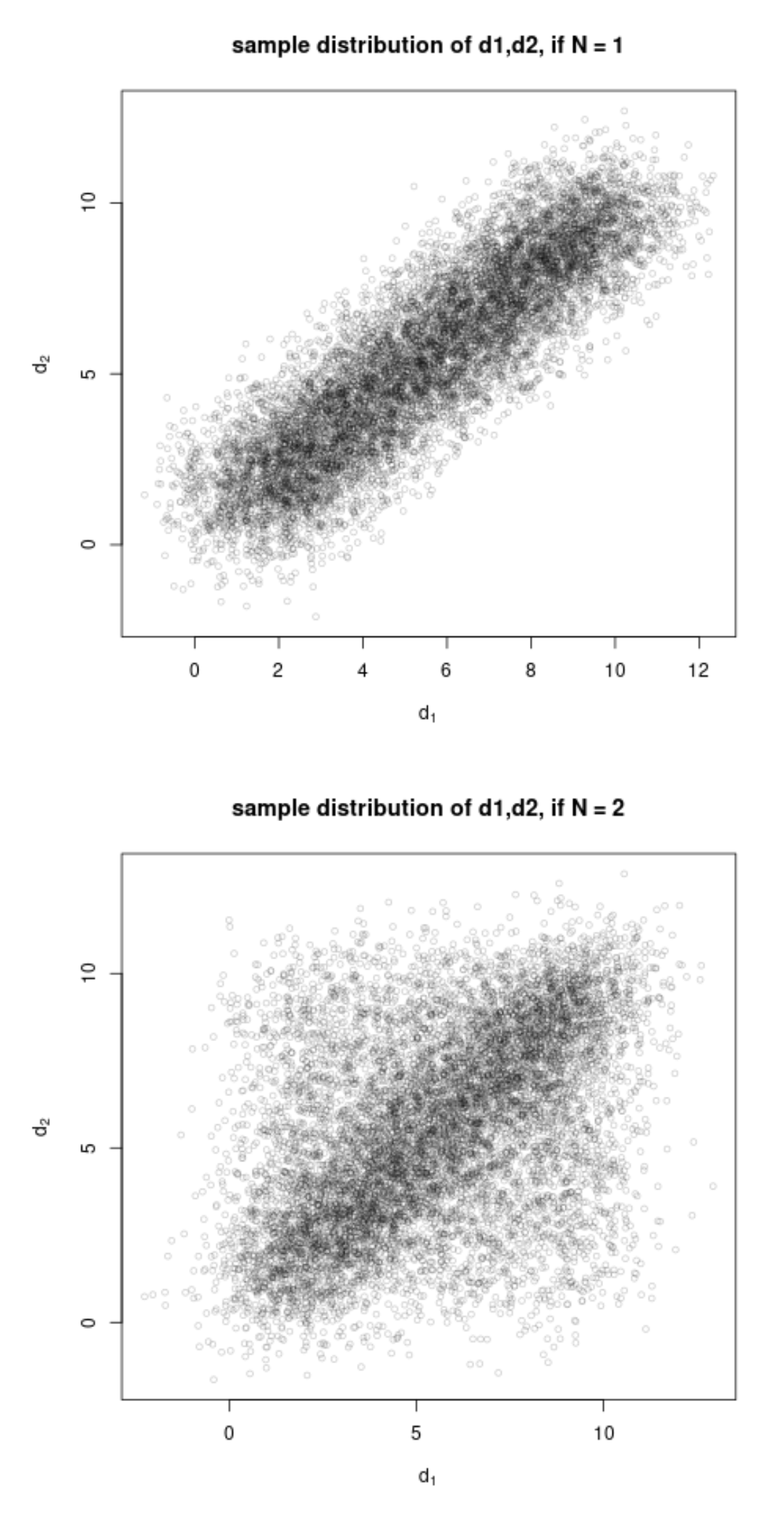
It is a bit difficult to compute exactly the likelihood, but we can estimate the distribution of the $d_i$ by using simulations, which is done to create the images below.

for $k\ge100$ our posterior mode would be $N=100$. So basically our estimate always only depends on how many samples we choose to get

As you can see for the case $k=2$, for the two different hypotheses $N=1$ and $N=2$ you get different sample distributions of $d_1,d_2$ and there are observations that are more likely when $N=1$ than when $N=2$, and vice versa, there are observations that are more likely when $N=2$ than when $N=1$.

So it is not the case that the maximum posterior will automatically be for the largest $N$. If the true $N$ is small, then you are likely to observe an observation with a high relative likelihood for a small $N$. The larger the sample size $k$ the more likely and more high the relative likelihood will be.

Now assume a scenario where $k$ is small, particularly less than $100$, e.g. $k=10$. In this case, it seems to me that our best bet for $N$, i.e. the most probable value for $N$, is $N=k$ (because of the slightly larger prior for smaller $N$s).

In the case that the number of observations $k$ is smaller than the maximum $N$, then the likelihood still contains information and the posterior probabilities are not the same as the prior probabilities.

For the case $k=2$, the distribution of $d_1,d_2$ consists of two components: either they come from the same button (with the same $\mu_i$), or they come from a different button. Depending on $N$ these different components are differently mixed. If we observe two extreme values like $d_1$ very small and $d_2$ very large, then this is more likely the higher the value of $N$ and so an observation with $k=2$ can already provide information about values $N>2$ as the likelihood differs.

set.seed(1)
n = 10^4

sim_1 = function() {
    mu = runif(1,1,10)
    d = rnorm(2,mu)
    return(d)
}

sim_2 = function() {
    mu = runif(2,1,10)
    selected = sample(1:2,2,replace = TRUE)
    d = rnorm(2,mu[selected])
    return(d)
}

D_1 = replicate(n, sim_1())
plot(t(D_1), 
     main = "sample distribution of d1,d2, if N = 1", 
     xlab = expression(d[1]),
     ylab = expression(d[2]),
     xlim = c(-2,13), ylim = c(-2,13),
     pch = 21, cex = 0.7, col = rgb(0,0,0,0.2))

D_2 = replicate(n, sim_2())
plot(t(D_2),
     main = "sample distribution of d1,d2, if N = 2", 
     xlab = expression(d[1]),
     ylab = expression(d[2]),
     xlim = c(-2,13), ylim = c(-2,13),
     pch = 21, cex = 0.7, col = rgb(0,0,0,0.2))

Answer 2

This, however, seems quite counter-intuitive to me, because (for small 𝑘) our inference only depends on our will regarding how many data points we want to generate!

Yes, but only because we're falling back on our prior that $N$ is small.

We can predictively manipulate our inference regardless of what data we will get. If I decide to bug the person in the room one more time, I know beforehand that my best estimate would be 𝑁=𝑘+1.

This is not necessarily true. For example, if you observe $d_1 = 103.2$ and $d_2 = 102.9$, the posterior becomes much more concentrated on $N=1$. More generally, the more data that is clumped together (recall that $\sigma = 1$, but $\mu_i \sim \text{Uniform}(1, 10^6)$), the more likely $N$ is to be small, where as the more "uniquely clustered" values we observe, the more likely it is for $N$ to be large.

In the case that $N >> k$, then it becomes fairly likely that all $d_i$ will belong to a unique cluster, and our posterior best guess for $N$ will be something like $k$ or $k+1$. But this paradox is nothing more than a combination of a bad prior + bad sampling strategy: our prior dictated that we believed $N$ was small, so we thought it would be okay to use a small $k$ so we're trying to determine how many clusters exist by using a sample whose size is smaller than the true number of clusters!

Answer 3

This one already has a few correct answers, but I think the intuition could be stronger. To start, let's set aside the noise temporarily, and assume that we can observe the $\mu_i$ values directly.

• After $k=1$ sample, we will have observed one unique value of $\mu$.
• On our second sample we will either have seen the same value again, or a new value.
  • If it's a new value we know that $N \geq 2$, at least. Since our prior is that $N$ is small, the most likely value is $N = 2$.
  • If it's the same value again, all we know is that $N \geq 1$, so $N = 1$ is most likely.
• More generally, after $k$ samples, we'll have observed $j$ unique values of $\mu$, where $j \leq k$. This indicates that $N \geq j$, and so due to the prior, $N = j$ is most likely.

Now, add back in the noise. $j$ is no longer observed directly but must be estimated, $\hat j$ based on the clustering of the observations. However, whatever way you estimate it, $\hat j \leq k$, and so the most likely value of $N$ remains $\leq k$.

Answer 4

We can predictively manipulate our inference regardless of what data we will get. If I decide to bug the person in the room one more time, I know beforehand that my best estimate would be N=k+1 . So I don't even need to ask the person anymore. I can already update my belief!

As Cliff noted, this isn't necessarily true. Assuming $k<N$ samples with $k$ different results $d_1,...,d_k$, you're always equally likely to get $d_{k+1}$ very close to one of the previous $k$ samples. This is true even for a certain range of $k>N$ values, as there's no guarantee that upon hitting $k=N$ requests you have been "exposed" to all $N$ options. The only thing that is guaranteed here is that for $K\ge N+1$ you have at least one cluster with two or more samples, due to the pigeonhole principle.

---

Taking no assumptions other than $N\le100$, you can solve this with Bayesian GMM and the Gibbs sampling algorithm. As you have known variance for the Gaussian models themselves and a strong assumption regarding the mixture probabilities. However we still take the probabilities vector $\pi$ as unknown so we don't limit ourselves to a fixed number of clusters (you'll see later why this works).

We denote $\theta=\{\pi,\{\mu_i\}_{i=1}^{100}\}$ our vector of parameters. An initial prior for $\pi$ would be $\pi\sim Dirichlet(\alpha_1,...,\alpha_{100})$. Of course $\forall i:\alpha_i>0, \pi_i\ge0, \sum_i\pi_i=1$. As you have a uniform assumption regarding the identities in the keystroke, you might want to take here $\alpha_1=...=\alpha_{100}$ and give it a high value (which reflects your high certainty in the Uniform manner).

Next the expectation vector with prior $\mu_i\sim U[1,10^6]$. Using the Bayes theorem we get $P(\mu|D)\propto P(D|\mu)P(\mu)$ (the denominator is a normalization constant which we can overlook for the moment). As the likelihood $P(D|\mu)$ is Gaussian and the prior $P(\mu)$ is uniform, the posterior $P(\mu|D)$ is a truncated Gaussian.

We start by choosing initial values for $\pi_i,\mu_i$ (for all $i$ values) and denote them $\pi_i^{(0)},\mu_i^{(0)}$. We then work iteratively, at each iteration $t+1$ we calculate the following steps, each step is calculated for all $k$ samples:

1. Responsibility $q_{ji}^{(t+1)}$ is the predicted probability of the sample $D_j$ belonging to the $i^{th}$ cluster after step $t$: $$q_{ji}^{(t+1)}=\frac{\pi_i^{(t)}\mathcal{N}(D_j;\mu_i^{(t)},1)}{\sum_{i=1}^N \pi_i^{(t)}\mathcal{N}(D_j;\mu_i^{(t)},1)}$$

2. Affiliation $$k_j^{(t+1)}\sim Multinomial \left(q_{j1}^{(t+1)},q_{j2}^{(t+1)},...,q_{jN}^{(t+1)}\right)$$

3. Cluster sizes: $$N_i^{(t+1)}=\sum_{j=1}^k\mathbb{I}\{k_j^{(t+1)}=j\}$$

4. Sampling the probabilities vector: $$(\pi^{(t+1)}|k^{(t+1)},D)\sim Dirichlet\left(N_1^{(t+1)}+\alpha_1,...,N_N^{(t+1)}+\alpha_N\right)$$

5. Calculating the expectations vector: Let $D^{i,(t+1)}$ be the subset of samples belonging to the $i^{th}$ cluster at this step: $$(\mu_i^{(t+1)}|k^{(t+1)},D^{i,(t+1)})=\frac{1}{N_i^{(t+1)}}\sum D^{i,(t+1)}$$

What happens eventually is that if the actual number of clusters is smaller that what we've initialized to, we'll get those clusters with 0 members and close to 0 mixture probability. You can also verify the number of clusters using the evidence function. Upon receiving a new sample $k+1$ you can re-run the whole process or (with some risks) initialize to the previous values.

Note that for the whole process, we have sticked with the basic assumptions and took nothing more.