It would be more correct to say you are fitting a model of the form
$$
g(\mu_i) = \mathbf{A}_i \boldsymbol{\beta} + f_1(x_{1i})
$$
as the MRF is the function $f_1$. Your definition separates the model matrix for the parametric terms from the model matrix for the smooth. Like any penalized spline, once we've evaluated the basis functions and computed their associated penalty matrix $\mathbf{S}$, we have a model matrix for the smooth $\mathbf{X}$ and we might as well combine it in with model matrix $\mathbf{A}$, and augment $\boldsymbol{\beta}$ such that it includes the coefficients for the spline basis functions as well as the parametric terms. At this point, the model is really just a fancy GLM with penalties on (typically [1]) a subset of $\boldsymbol{\beta}$ that are associated with the smooth(s):
$$
g(\mu_i) = \mathbf{X}_i \boldsymbol{\beta}
$$
So, what's the function $f$?
It might help to think about how random effects get represented in penalized spline form, as random effects are a special case of an intrinsic Gaussian Markov random field. A penalized spline is effectively composed of two things:
- the basis functions $b_{jk}(\mathbf{x})$ evaluated at the covariate values $\mathbf{x}_j$, yielding the model matrix and
- the penalty matrix $\mathbf{S}$ of the basis functions
The model matrix for a random effect is just a binary indicator matrix with $n_{\text{subject}}$ columns and $n$ rows, where the rows simply indexes to which of the $n_{\text{subject}}$ each row belongs. The penalty matrix $\mathbf{S}$ for a random effect in penalized spline form is an identity matrix $\mathbf{I}$. This means that we shrink (penalize) the coefficient for each subject towards the overall mean of the response (the model constant term, the "intercept") but there's no correlation among the subjects; each is penalized independently of the others (because of the 0 off-diagonal elements).
Let's explore this a little using R and mgcv. We'll also use an in-development package that Eric Pedersen and I are working on, to make working with the "mrf" basis in mgcv easier; it's not on CRAN so you'll need to install from GitHub if you want to follow along and explore more:
# install.packages("remotes")
# remotes::install_github("eric-pedersen/MRFtools")
library("mgcv")
library("MRFtools")
library("dplyr")
library("ggplot2")
library("patchwork")
We define some dummy data to work with too
set.seed(1)
i <- 1:10
f <- factor(i, levels = i)
df <- data.frame(y = (0.4 * i) + rnorm(length(i)), f = f, i = i)
This is what the random effect penalty looks like:
mrf_penalty(f, type = "individual") |> as.matrix()
> mrf_penalty(f, type = "individual") |> as.matrix()
   1 2 3 4 5 6 7 8 9 10
1  1 0 0 0 0 0 0 0 0  0
2  0 1 0 0 0 0 0 0 0  0
3  0 0 1 0 0 0 0 0 0  0
4  0 0 0 1 0 0 0 0 0  0
5  0 0 0 0 1 0 0 0 0  0
6  0 0 0 0 0 1 0 0 0  0
7  0 0 0 0 0 0 1 0 0  0
8  0 0 0 0 0 0 0 1 0  0
9  0 0 0 0 0 0 0 0 1  0
10 0 0 0 0 0 0 0 0 0  1
The model matrix looks the same too because we have one observation per subject here. If we use a lower level mgcv tool we can see this
S_re <- smoothCon(s(f, bs = "re"), data = df)[[1]]
First the model matrix:
> S_re$X
   f1 f2 f3 f4 f5 f6 f7 f8 f9 f10
1   1  0  0  0  0  0  0  0  0   0
2   0  1  0  0  0  0  0  0  0   0
3   0  0  1  0  0  0  0  0  0   0
4   0  0  0  1  0  0  0  0  0   0
5   0  0  0  0  1  0  0  0  0   0
6   0  0  0  0  0  1  0  0  0   0
7   0  0  0  0  0  0  1  0  0   0
8   0  0  0  0  0  0  0  1  0   0
9   0  0  0  0  0  0  0  0  1   0
10  0  0  0  0  0  0  0  0  0   1
attr(,"assign")
 [1] 1 1 1 1 1 1 1 1 1 1
attr(,"contrasts")
attr(,"contrasts")$f
[1] "contr.treatment"
and now the penalty matrix $\mathbf{X}_j$ for the penalized spline representation of a random effect
> S_re$S
[[1]]
      [,1] [,2] [,3] [,4] [,5] [,6] [,7] [,8] [,9] [,10]
 [1,]    1    0    0    0    0    0    0    0    0     0
 [2,]    0    1    0    0    0    0    0    0    0     0
 [3,]    0    0    1    0    0    0    0    0    0     0
 [4,]    0    0    0    1    0    0    0    0    0     0
 [5,]    0    0    0    0    1    0    0    0    0     0
 [6,]    0    0    0    0    0    1    0    0    0     0
 [7,]    0    0    0    0    0    0    1    0    0     0
 [8,]    0    0    0    0    0    0    0    1    0     0
 [9,]    0    0    0    0    0    0    0    0    1     0
[10,]    0    0    0    0    0    0    0    0    0     1
If we plug all this together into a GAM we have
m_re <- gam(y ~ s(f, bs = "re"), data = df)
Which (apart from the row and column names) is what we created with mrf_penalty() earlier.
You'll need a recent version of mgcv for that to work, because up until version 1.9.0 you couldn't have more coefficients than data and here we're estimating an intercept plus 10 coefficients for the the 10 subjects (levels) in f:
r$> length(coef(m_re))
[1] 11

r$> nrow(df)
[1] 10
If we extract the complete model matrix for the entire GAM we see the combination of the two model matrices $\mathbf{A}$ and $\mathbf{X}$, where in this case the parametric model matrix $\mathbf{A}$ is just a vector of 1s
r$> model.matrix(m_re)
   (Intercept) s(f).1 s(f).2 s(f).3 s(f).4 s(f).5 s(f).6 s(f).7 s(f).8 s(f).9 s(f).10
1            1      1      0      0      0      0      0      0      0      0       0
2            1      0      1      0      0      0      0      0      0      0       0
3            1      0      0      1      0      0      0      0      0      0       0
4            1      0      0      0      1      0      0      0      0      0       0
5            1      0      0      0      0      1      0      0      0      0       0
6            1      0      0      0      0      0      1      0      0      0       0
7            1      0      0      0      0      0      0      1      0      0       0
8            1      0      0      0      0      0      0      0      1      0       0
9            1      0      0      0      0      0      0      0      0      1       0
10           1      0      0      0      0      0      0      0      0      0       1
attr(,"model.offset")
[1] 0
So the $f_j(x_i)$ trm in the model equation we wrote out earlier results in $k$ binary columns being added to the model matrix, which you called an incidence matrix.
Going from the random effect representation to the more general MRF follows naturally, except we're going to be creating fancier penalty matrices. The nice thing about the way Simon implemented the "mrf" basis in mgcv is that while it is a pain to specify the neighbourhood object, rather than directly use a sf object say, that we can specify the penalty directly allows for a much richer set of MRFs to be represented. Which is where MRFtools comes in.
This is the MRF for a first-order random walk:
mrf_penalty(i) |> as.matrix()
> mrf_penalty(i) |> as.matrix()
    1  2  3  4  5  6  7  8  9 10
1   1 -1  0  0  0  0  0  0  0  0
2  -1  2 -1  0  0  0  0  0  0  0
3   0 -1  2 -1  0  0  0  0  0  0
4   0  0 -1  2 -1  0  0  0  0  0
5   0  0  0 -1  2 -1  0  0  0  0
6   0  0  0  0 -1  2 -1  0  0  0
7   0  0  0  0  0 -1  2 -1  0  0
8   0  0  0  0  0  0 -1  2 -1  0
9   0  0  0  0  0  0  0 -1  2 -1
10  0  0  0  0  0  0  0  0 -1  1
which denotes the dependence of $x_t$ on $x_{t-1}$ (and hence also a relationship between $x_t$ and $x_{t+1}$. The -1s in the $i$th row indicate the neighbours of the $i$th observation. For example, row 2 ($i = 2$), is a neighbour of observations 1 and 3. The diagonal values in the matrix give the number of neighbours of each observation, which here is 2 except for the start and end observations.
The key thing to note here is that we defined the penalty matrix as representing the neighbours of each observation. The same thing happens with areal spatial data, where we define neighbours as those regions sharing a border. But if you can represent the data as an undirected graph, we can turn it into an MRF penalty that mgcv can estimate (as long as the penalty doesn't depend on other parameters, which an AR($p$) process would for example).
Here I'll use the US census data on median income per census tract in Orange County, CA, just as an example that was easy to come across
library(tidycensus)
library(tigris)
options(tigris_use_cache = TRUE)

orange <- get_acs(
  state = "CA",
  county = "Orange",
  geography = "tract",
  variables = "B19013_001",
  geometry = TRUE,
  year = 2020
)
This returns an sf tibble (fancy data frame containing the geometry for plotting)
r$> orange
Simple feature collection with 614 features and 5 fields (with 1 geometry empty)
Geometry type: MULTIPOLYGON
Dimension:     XY
Bounding box:  xmin: -118.1154 ymin: 33.38779 xmax: -117.4133 ymax: 33.94764
Geodetic CRS:  NAD83
First 10 features:
         GEOID                                            NAME   variable
1  06059110603 Census Tract 1106.03, Orange County, California B19013_001
2  06059011503  Census Tract 115.03, Orange County, California B19013_001
3  06059001102   Census Tract 11.02, Orange County, California B19013_001
4  06059021812  Census Tract 218.12, Orange County, California B19013_001
5  06059001301   Census Tract 13.01, Orange County, California B19013_001
6  06059088701  Census Tract 887.01, Orange County, California B19013_001
7  06059001101   Census Tract 11.01, Orange County, California B19013_001
8  06059110117 Census Tract 1101.17, Orange County, California B19013_001
9  06059110106 Census Tract 1101.06, Orange County, California B19013_001
10 06059099905  Census Tract 999.05, Orange County, California B19013_001
   estimate   moe                       geometry
1     56563 13103 MULTIPOLYGON (((-118.0096 3...
2    101800 10306 MULTIPOLYGON (((-117.8984 3...
3     99286 18207 MULTIPOLYGON (((-117.9765 3...
4    133494  8958 MULTIPOLYGON (((-117.8184 3...
5     75994 18045 MULTIPOLYGON (((-117.9766 3...
6     54759  7682 MULTIPOLYGON (((-117.9673 3...
7    101500 10792 MULTIPOLYGON (((-117.9765 3...
8    103368 14136 MULTIPOLYGON (((-118.0632 3...
9    107045 11870 MULTIPOLYGON (((-118.063 33...
10    79857 21573 MULTIPOLYGON (((-118.0412 3...
We create the penalty directly from the orange sf object, and (currently) we have to explicitly set the node labels of the graph (the census tract names here) so that they will match the levels of the factor used to set up the smooth
orange_pen <- orange |>
  mrf_penalty(node_labels = orange$NAME)
and now we can fit the model. We need to convert the NAME variable to a factor otherwise mgcv will throw an error
levs <- with(orange, unique(NAME))
orange2 <- orange |>
  mutate(fNAME = factor(NAME, levels = levs))

m_orange <- gam(estimate ~
    s(fNAME, bs = "mrf", xt = list(penalty = orange_pen)),
  data = orange2,
  method = "REML",
  drop.unused.levels = FALSE,
  na.action = na.exclude)
Which takes a little while as we're fitting the full rank MRF (one coefficient per region). The resulting fit is good:
summary(m_orange)
r$> summary(m_orange)

Family: gaussian
Link function: identity

Formula:
estimate ~ s(fNAME, bs = "mrf", xt = list(penalty = orange_pen))

Parametric coefficients:
            Estimate Std. Error t value Pr(>|t|)
(Intercept) 101316.7      619.6   163.5   <2e-16 ***
---
Signif. codes:  0 ‘***’ 0.001 ‘**’ 0.01 ‘*’ 0.05 ‘.’ 0.1 ‘ ’ 1

Approximate significance of smooth terms:
         edf Ref.df     F p-value
s(fNAME) 408  533.7 5.195  <2e-16 ***
---
Signif. codes:  0 ‘***’ 0.001 ‘**’ 0.01 ‘*’ 0.05 ‘.’ 0.1 ‘ ’ 1

Rank: 613/614
R-sq.(adj) =  0.825   Deviance explained = 94.2%
-REML = 7116.3  Scale est. = 2.3459e+08  n = 611
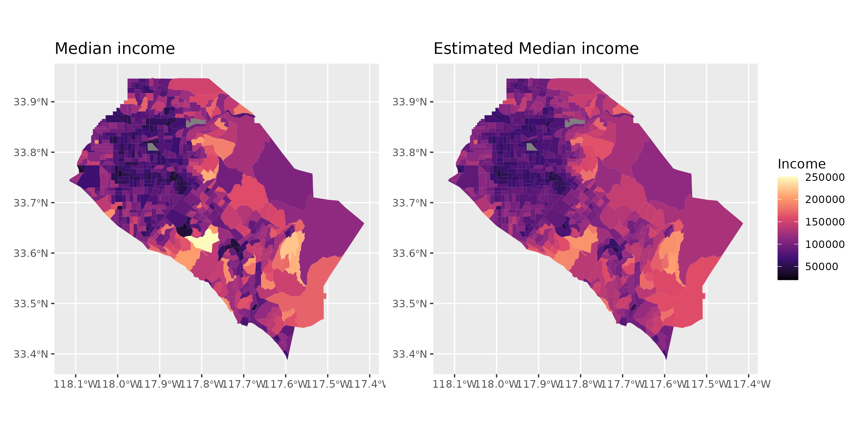
We can plot the estimate income by taking the fitted values and adding them to the object used to fit the model
orange2 <- orange2 |>
  mutate(.fitted = fitted(m_orange))

cb <- guide_colorbar(title = "Income")
fill_sc <- scale_fill_viridis_c(option = "magma",
  guide = cb,
  limits = c(20000, 251000))

p_income <- orange |>
  ggplot(aes(fill = estimate)) +
  geom_sf(color = NA) +
  fill_sc +
  labs(title = "Median income")

p_fitted <- orange2 |>
  ggplot(aes(fill = .fitted)) +
  geom_sf(color = NA) +
  fill_sc +
  labs(title = "Estimated Median income")

p_income + p_fitted + plot_layout(guides = "collect")

It's obviously not perfect, but a large part of the variation in median income can be "explained" by the crude spatial information about which tracts are neighbours of one another. (Of course we're not actually explaining anything here!)
The first 10 rows and columns of orange_pen (after stripping the row/column names) are
      [,1] [,2] [,3] [,4] [,5] [,6] [,7] [,8] [,9] [,10]
 [1,]    4    0    0    0    0    0    0    0    0     0
 [2,]    0    5    0    0    0    0    0    0    0     0
 [3,]    0    0    3    0   -1    0   -1    0    0     0
 [4,]    0    0    0    5    0    0    0    0    0     0
 [5,]    0    0   -1    0    7    0    0    0    0     0
 [6,]    0    0    0    0    0    7    0    0    0     0
 [7,]    0    0   -1    0    0    0    3    0    0     0
 [8,]    0    0    0    0    0    0    0    4   -1     0
 [9,]    0    0    0    0    0    0    0   -1    6     0
[10,]    0    0    0    0    0    0    0    0    0     4
We see that tract 3 is a neighbour of tracts 5 and 7 (an another tract outside the first 10 shown). Tract 5 has 7 neighbours, etc.
The form of the penalty matrix induces neighbouring tracts to be similar to one another - i.e. spatially smooth. It does this because of the negative values (-1) in the off diagonals - these will reduce the overall wiggliness penalty if neighbouring tracts have similar coefficients, and we estimate the coefficients as those that maximise the penalised likelihood of the data given the model. Hence we're balancing the fit to the data with the complexity of the MRF when estimating the coefficients.
Contrast this model that induces spatial smoothness with a random effect version, which just estimates independent penalized coefficients for each tract, ignoring their spatial arrangement:
m_orange_re <- gam(estimate ~ s(fNAME, bs = "re"),
  data = orange2,
  method = "REML",
  drop.unused.levels = FALSE,
  na.action = na.exclude)

orange2 <- orange2 |>
  mutate(.fitted_re = fitted(m_orange_re))
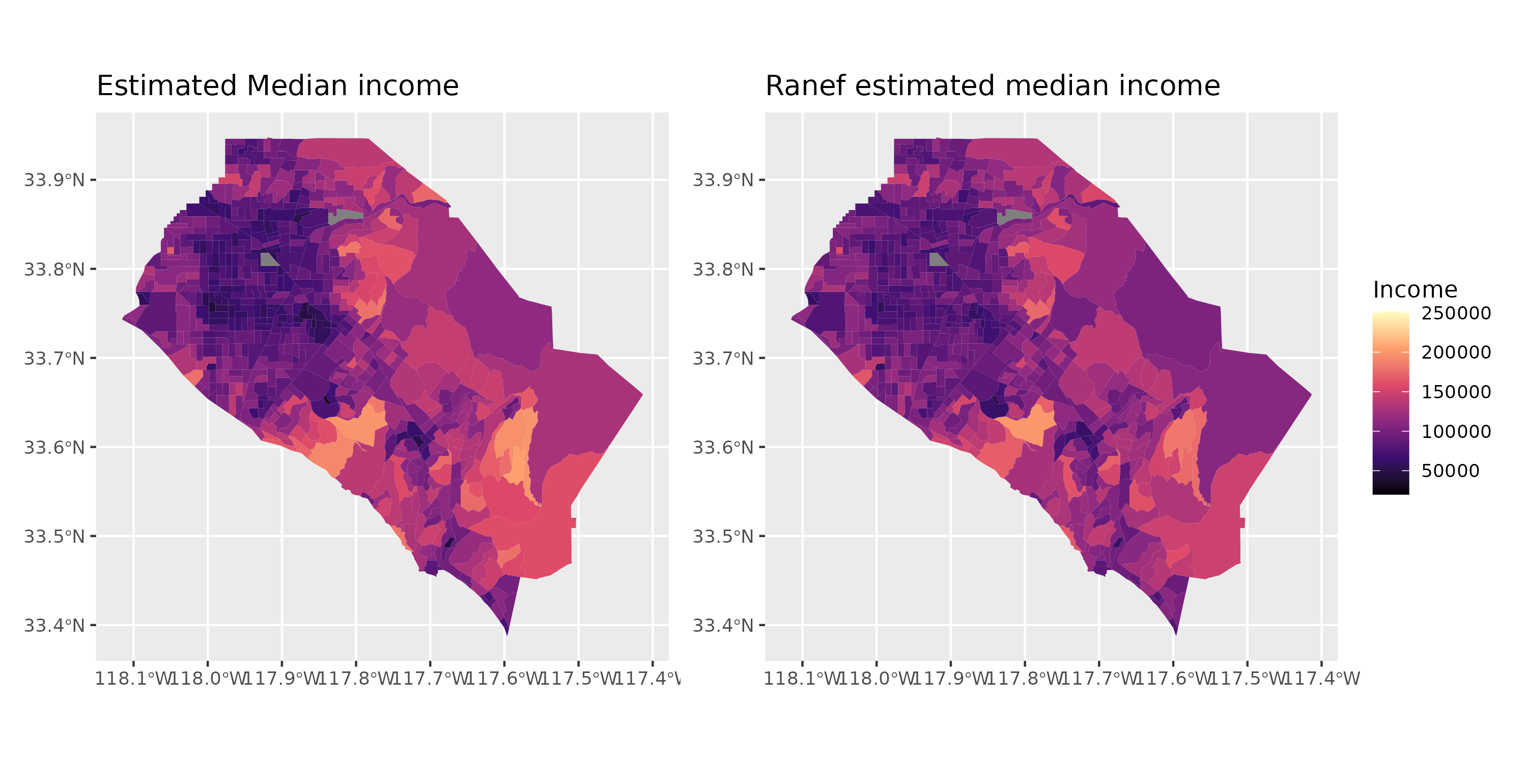
and which doesn't do quite as good a job of fitting the data as the MRF
> summary(m_orange_re)

Family: gaussian
Link function: identity

Formula:
estimate ~ s(fNAME, bs = "re")

Parametric coefficients:
            Estimate Std. Error t value Pr(>|t|)
(Intercept)   101317       1482   68.36   <2e-16 ***
---
Signif. codes:  0 ‘***’ 0.001 ‘**’ 0.01 ‘*’ 0.05 ‘.’ 0.1 ‘ ’ 1

Approximate significance of smooth terms:
           edf Ref.df     F p-value
s(fNAME) 402.5    610 1.939  <2e-16 ***
---
Signif. codes:  0 ‘***’ 0.001 ‘**’ 0.01 ‘*’ 0.05 ‘.’ 0.1 ‘ ’ 1

R-sq.(adj) =   0.66   Deviance explained = 88.4%
-REML = 7279.1  Scale est. = 4.5658e+08  n = 611
although the estimated incomes are similar
p_re <- orange2 |>
  ggplot(aes(fill = .fitted_re)) +
  geom_sf(color = NA) +
  fill_sc +
  labs(title = "Ranef estimated median income", fill = "Income")

p_fitted + p_re + plot_layout(guides = "collect")

Final note, I have kept the family as the default family = gaussian() to keep model estimation times down here, but it's unlikely that income is (conditionally) Gaussian. In fact the model diagnostics for both models are terrible (and remain terrible if we try to do something more complex like use family = Gamma(link = "log")) largely because we're ignoring every causal factor except the purely spatial component. So don't read anything into the models themselves.
As for references, I would read (if you have access to it) Simon's book a referenced on ?mrf, especially section 5.8.1 (page 240-241). Beyond that, Fahrmier et al (2012) have another good description of these kinds of models with other examples.
Footnote
- You can penalize all the coefficients if you want through a combination of
paraPen and select = TRUE, depending on specific details of the basis that are not necessary here


