Use Gaussian RBF kernel for mapping of 2D data to 3D

Question

I am working on SVMs and try to get all the concepts involved. For instance, the kernel mapping. I would like to construct some parts of the algorithm by myself, to understand what is happening.

My goal is to create a mapping as in this picture (taken from here)

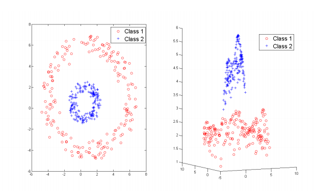
I do not fully understand what the input and output values of the kernel are; to map the data points to the 3rd dimension, the output should be the Z-values, right? And the input are (vectors of) the X and Y-values?

My (matlab) code to get the z-values is:

z = exp(-( (abs(x-y).^2)./ (2*gamma^2) ));

But the z-values are just a bell-curve, us such:

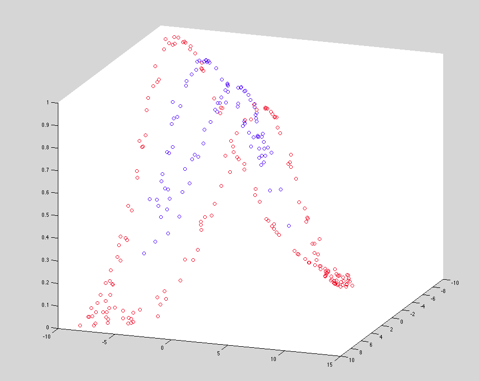
I don't really know what I am doing wrong, but I think I confuse the concepts of kernel and (implicit/explicit) mapping.

How can I construct a (matlab) function that maps the 2D data to 3D space, using the Gaussian Radial Basis Function?

-- Edit -- Thanks to user27840 I made it work, with the following matlab code:

gamma = 2;
D = squareform( pdist(data, 'euclidean') );
D = exp(-(D .^ 2) ./ ( 2*gamma^2));
z = sum(D);

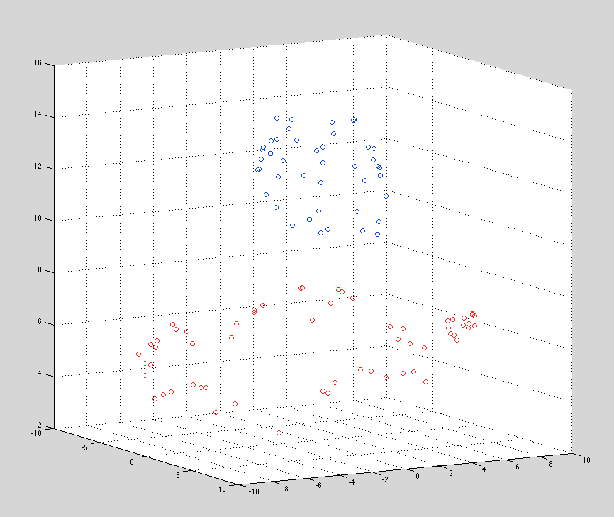
This results in the following 3D plot, from original 2D data:

-- Edit2: -- For those who are interested in one-class support vector machines; I wrote a blog post about it, using the answer from this thread: Introduction to one-class Support Vector Machine

Answer 1

I believe RBF projects the data into 3D space by centering a three dimensional bump (an un-normalized Gaussian) on top of each data point. The width of the bumps is given by the $gamma$ parameter.

These bumps overlap, so to figure out the z value at particular place you need to sum over all of the data points. If instead of $x, y$ we use $x_1, x_2$, and index all of the data points as $\mathbf{x}_i$ then the formula for to calculate the projection is:

$ z(\mathbf{x}) = \sum_{i=1}^{n} \exp\{ - \frac{ \| \mathbf{x} - \mathbf{x_i} \|^2}{2 \gamma^2 } \} $

Where $\mathbf{x}$ and $\mathbf{x}_i$ are two dimensional vectors and $\| \mathbf{x} - \mathbf{x}_i \|$ is the Euclidean distance between them.

That is, to find the z value at each point, you need to sum across all the data points.