27
$\begingroup$

Almost everything I read about linear regression and GLM boils down to this: $y = f(x,\beta)$ where $f(x,\beta)$ is a non-increasing or non-decreasing function of $x$ and $\beta$ is the parameter you estimate and test hypotheses about. There are dozens of link functions and transformations of $y$ and $x$ to make $y$ a linear function of $f(x,\beta)$.

Now, if you remove the non-increasing/non-decreasing requirement for $f(x,\beta)$, I know of only two choices for fitting a parametric linearized model: trig functions and polynomials. Both create artificial dependence between each predicted $y$ and the entire set of $X$, making them a very non-robust fit unless there are prior reasons to believe that your data actually are generated by a cyclical or polynomial process.

This is not some kind of esoteric edge case. It's the actual, common-sense relationship between water and crop yields (once the plots are deep enough under water, crop yields will start diminishing), or between calories consumed at breakfast and performance on a math quiz, or number of workers in a factory and the number of widgets they produce... in short, almost any real life case for which linear models are used but with the data covering a wide enough range that you go past diminishing returns into negative returns.

I tried looking for the terms 'concave', 'convex', 'curvilinear', 'non-monotonic', 'bathtub', and I forget how many others. Few relevant questions and even fewer usable answers. So, in practical terms, if you had the following data (R code, y is a function of continuous variable x and discrete variable group):

updown<-data.frame(y=c(46.98,38.39,44.21,46.28,41.67,41.8,44.8,45.22,43.89,45.71,46.09,45.46,40.54,44.94,42.3,43.01,45.17,44.94,36.27,43.07,41.85,40.5,41.14,43.45,33.52,30.39,27.92,19.67,43.64,43.39,42.07,41.66,43.25,42.79,44.11,40.27,40.35,44.34,40.31,49.88,46.49,43.93,50.87,45.2,43.04,42.18,44.97,44.69,44.58,33.72,44.76,41.55,34.46,32.89,20.24,22,17.34,20.14,20.36,24.39,22.05,24.21,26.11,28.48,29.09,31.98,32.97,31.32,40.44,33.82,34.46,42.7,43.03,41.07,41.02,42.85,44.5,44.15,52.58,47.72,44.1,21.49,19.39,26.59,29.38,25.64,28.06,29.23,31.15,34.81,34.25,36,42.91,38.58,42.65,45.33,47.34,50.48,49.2,55.67,54.65,58.04,59.54,65.81,61.43,67.48,69.5,69.72,67.95,67.25,66.56,70.69,70.15,71.08,67.6,71.07,72.73,72.73,81.24,73.37,72.67,74.96,76.34,73.65,76.44,72.09,67.62,70.24,69.85,63.68,64.14,52.91,57.11,48.54,56.29,47.54,19.53,20.92,22.76,29.34,21.34,26.77,29.72,34.36,34.8,33.63,37.56,42.01,40.77,44.74,40.72,46.43,46.26,46.42,51.55,49.78,52.12,60.3,58.17,57,65.81,72.92,72.94,71.56,66.63,68.3,72.44,75.09,73.97,68.34,73.07,74.25,74.12,75.6,73.66,72.63,73.86,76.26,74.59,74.42,74.2,65,64.72,66.98,64.27,59.77,56.36,57.24,48.72,53.09,46.53),
                   x=c(216.37,226.13,237.03,255.17,270.86,287.45,300.52,314.44,325.61,341.12,354.88,365.68,379.77,393.5,410.02,420.88,436.31,450.84,466.95,477,491.89,509.27,521.86,531.53,548.11,563.43,575.43,590.34,213.33,228.99,240.07,250.4,269.75,283.33,294.67,310.44,325.36,340.48,355.66,370.43,377.58,394.32,413.22,428.23,436.41,455.58,465.63,475.51,493.44,505.4,521.42,536.82,550.57,563.17,575.2,592.27,86.15,91.09,97.83,103.39,107.37,114.78,119.9,124.39,131.63,134.49,142.83,147.26,152.2,160.9,163.75,172.29,173.62,179.3,184.82,191.46,197.53,201.89,204.71,214.12,215.06,88.34,109.18,122.12,133.19,148.02,158.72,172.93,189.23,204.04,219.36,229.58,247.49,258.23,273.3,292.69,300.47,314.36,325.65,345.21,356.19,367.29,389.87,397.74,411.46,423.04,444.23,452.41,465.43,484.51,497.33,507.98,522.96,537.37,553.79,566.08,581.91,595.84,610.7,624.04,637.53,649.98,663.43,681.67,698.1,709.79,718.33,734.81,751.93,761.37,775.12,790.15,803.39,818.64,833.71,847.81,88.09,105.72,123.35,132.19,151.87,161.5,177.34,186.92,201.35,216.09,230.12,245.47,255.85,273.45,285.91,303.99,315.98,325.48,343.01,360.05,373.17,381.7,398.41,412.66,423.66,443.67,450.39,468.86,483.93,499.91,511.59,529.34,541.35,550.28,568.31,584.7,592.33,615.74,622.45,639.1,651.41,668.08,679.75,692.94,708.83,720.98,734.42,747.83,762.27,778.74,790.97,806.99,820.03,831.55,844.23),
                   group=factor(rep(c('A','B'),c(81,110))));

plot(y~x,updown,subset=x<500,col=group);
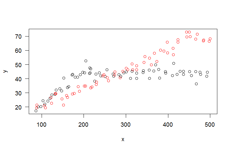
Scatterplot

You might first try a Box-Cox transformation and see if it made mechanistic sense, and failing that, you might fit a nonlinear least squares model with a logistic or asymptotic link function.

So, why should you give up parametric models completely and fall back on a black-box method like splines when you find out that the full dataset looks like this...

plot(y~x,updown,col=group);

My questions are:

  • What terms should I search for in order to either find link functions that represent this class of functional relationships?

or

  • What should I read and/or search for in order to teach myself how to design link functions to this class of functional relationships or extend existing ones that currently are only for monotonic responses?

or

  • Heck, even what StackExchange tag is most appropriate for this type of question!
$\endgroup$
10
  • 5
    $\begingroup$ I have no idea what you're asking. You want to fit a non-monotonic function of $x$... what exactly is your problem with polynomial regression or sine regression again?? Also... "link function"... you keep using that word... I do not think it means what you think it means. $\endgroup$ Commented Jul 11, 2013 at 2:43
  • 6
    $\begingroup$ (1) Your R code has syntax errors: group should not be quoted. (2) The plot is beautiful: the red dots exhibit a linear relationship while the black ones could be fit in several ways, including a piecewise linear regression (obtained with a changepoint model) and possibly even as an exponential. I am not recommending these, however, because modeling choices ought to be informed by an understanding of what produced the data and motivated by theories in relevant disciplines. They might be a better start for your research. $\endgroup$
    – whuber
    Commented Jul 11, 2013 at 2:54
  • 1
    $\begingroup$ @whuber thanks! Fixed the code. Regarding theoretical motivation: where do these come from in the first place? My bench scientist collaborators will happily dichotomize the predictor variables and do t-tests on them. So it falls to me find a way to stop wasting data by finding a mathematical relationship that captures the transition from "y correlates positively with x" to "y has little response to x" to "y correlates negatively with x". Failing that, I'll have to recapitulate what, e.g., Michaelis and Menten did when they found a relationship between enzyme, substrate, and product. $\endgroup$
    – f1r3br4nd
    Commented Jul 11, 2013 at 3:11
  • 3
    $\begingroup$ +1 for the provocative title and a followup that actually makes sense $\endgroup$ Commented Jul 11, 2013 at 5:31
  • 2
    $\begingroup$ I don't really understand the problem. I am most familiar with your crop yield/water example. There are (often quite complex) models available that are based on micro-meterology, soil physics, plant physiology, nutrient supply (fertilization), and so forth. You find them in the literature. If you fit an empirical model it can only approximate such a complex model over a limited range. It may be that a linear model is appropriate to answer your specific question, it may be that you need to be able to model saturation (use an appropriate non-linear function). $\endgroup$
    – Roland
    Commented Jul 11, 2013 at 9:54

5 Answers 5

60
$\begingroup$

The remarks in the question about link functions and monotonicity are a red herring. Underlying them seems to be an implicit assumption that a generalized linear model (GLM), by expressing the expectation of a response $Y$ as a monotonic function $f$ of a linear combination $X\beta$ of explanatory variables $X$, is not flexible enough to account for non-monotonic responses. That's just not so.


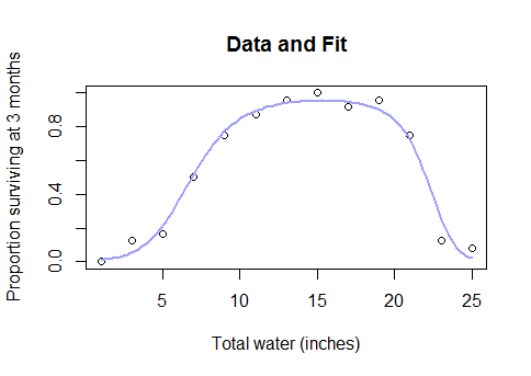
Perhaps a worked example will illuminate this point. In a 1948 study (published posthumously in 1977 and never peer-reviewed), J. Tolkien reported the results of a plant watering experiment in which 13 groups of 24 sunflowers (Helianthus Gondorensis) were given controlled amounts of water starting at germination through three months of growth. The total amounts applied varied from one inch to 25 inches in two-inch increments.

Figure 1

There is a clear positive response to the watering and a strong negative response to over-watering. Earlier work, based on hypothetical kinetic models of ion transport, had hypothesized that two competing mechanisms might account for this behavior: one resulted in a linear response to small amounts of water (as measured in the log odds of survival), while the other--an inhibiting factor--acted exponentially (which is a strongly non-linear effect). With large amounts of water, the inhibiting factor would overwhelm the positive effects of the water and appreciably increase mortality.

Let $\kappa$ be the (unknown) inhibition rate (per unit amount of water). This model asserts that the number $Y$ of survivors in a group of size $n$ receiving $x$ inches of water should have a $$\text{Binomial}\left(n, f(\beta_0 + \beta_1 x - \beta_2 \exp(\kappa x))\right)$$ distribution, where $f$ is the link function converting log odds back to a probability. This is a binomial GLM. As such, although it is manifestly nonlinear in $x$, given any value of $\kappa$ it is linear in its parameters $\beta_0$, $\beta_1$, and $\beta_2$. "Linearity" in the GLM setting has to be understood in the sense that $f^{-1}\left(\mathbb{E}[Y]\right)$ is a linear combination of these parameters whose coefficients are known for each $x$. And they are: they equal $1$ (the coefficient of $\beta_0$), $x$ itself (the coefficient of $\beta_1$), and $-\exp(\kappa x)$ (the coefficient of $\beta_2$).

This model--although it is somewhat novel and not completely linear in its parameters--can be fit using standard software by maximizing the likelihood for arbitrary $\kappa$ and selecting the $\kappa$ for which this maximum is largest. Here is R code to do so, beginning with the data:

water <- seq(1, 25, length.out=13)
n.survived <- c(0, 3, 4, 12, 18, 21, 23, 24, 22, 23, 18, 3, 2)
pop <- 24
counts <- cbind(n.survived, n.died=pop-n.survived)
f <- function(k) {
  fit <- glm(counts ~ water + I(-exp(water * k)), family=binomial)
  list(AIC=AIC(fit), fit=fit)
}
k.est <- optim(0.1, function(k) f(k)$AIC, method="Brent", lower=0, upper=1)$par
fit <- f(k.est)$fit

There are no technical difficulties; the calculation takes only 1/30 second.

Figure 2

The blue curve is the fitted expectation of the response, $\mathbb{E}[Y]$.

Obviously (a) the fit is good and (b) it predicts a non-monotonic relationship between $\mathbb{E}[Y]$ and $x$ (an upside-down "bathtub" curve). To make this perfectly clear, here is the follow-up code in R used to compute and plot the fit:

x.0 <- seq(min(water), max(water), length.out=100)
p.0 <- cbind(rep(1, length(x.0)), x.0, -exp(k.est * x.0))
logistic <- function(x) 1 - 1/(1 + exp(x))
predicted <- pop * logistic(p.0 %*% coef(fit))

plot(water, n.survived / pop, main="Data and Fit",
     xlab="Total water (inches)", 
     ylab="Proportion surviving at 3 months")
lines(x.0, predicted / pop, col="#a0a0ff", lwd=2)

The answers to the questions are:

What terms should I search for in order to either find link functions that represent this class of functional relationships?

None: that is not the purpose of the link function.

What should I ... search for in order to ... extend existing [link functions] that currently are only for monotonic responses?

Nothing: this is based on a misunderstanding of how responses are modeled.

Evidently, one should first focus on what explanatory variables to use or construct when building a regression model. As suggested in this example, look for guidance from past experience and theory.

$\endgroup$
8
  • 1
    $\begingroup$ awesome answer! Is this actual data tolkien from the novel? $\endgroup$ Commented Jul 12, 2013 at 17:15
  • 2
    $\begingroup$ @Cam The data didn't make it into the final cut :-). (The context is rather tongue-in-cheek, I'm afraid.) $\endgroup$
    – whuber
    Commented Jul 12, 2013 at 17:19
  • 1
    $\begingroup$ @whuber Great answer whuber! Any suggestions on how one would get the standard error or distribution of $\kappa$? $\endgroup$ Commented Dec 4, 2014 at 18:38
  • 7
    $\begingroup$ @Trynna That's a great question which I was trying to dodge :-). A profile likelihood approach is the first thing to come to mind: vary $\kappa$, refit the other parameters, and recompute the log likelihood. Plot twice this log likelihood against $\kappa$ and identify where its decrease is significant (referring to a $\chi^2(1)$ distribution). This will give a confidence interval which can be backed into something like a standard error if it looks sufficiently symmetric. If you want a distribution, you might elect a parametric bootstrap. $\endgroup$
    – whuber
    Commented Dec 4, 2014 at 18:47
  • 2
    $\begingroup$ @zipzapboing The example I give here is special because it was informed by an underlying theory. When such information is available, it can be a powerful guide to selecting a model. In many cases, though, there is no such information, or one only hopes that the expected response might vary monotonically with the regressors. Perhaps the most fundamental reason one might point to is the hope that the response varies differentiably with the regressors and that, for the range of regressors in the data, the change in derivative is small: a linear response would approximate that well. $\endgroup$
    – whuber
    Commented Sep 14, 2018 at 17:06
10
$\begingroup$

Looks guiltily at the dying plant on his desk....apparently not

In the comments, @whuber says that "modeling choices ought to be informed by an understanding of what produced the data and motivated by theories in relevant disciplines", to which you asked how one goes about doing this.

The Michaelis and Menten kinetics is actually a pretty useful example. Those equations can be derived by starting with some assumptions (e.g., the substrate is in equilibrium with its complex, the enzyme is not consumed) and some known principles (the law of mass action). Murray's Mathematical Biology: An Introduction walks through the derivation in chapter 6 (I would bet many other books do too!).

More generally, it helps to build up a "repertoire" of models and assumptions. I'm sure your field has some commonly-accepted, time-tested models. For example, if something is charging or discharging, I would reach for an exponential to model its voltage as a function of time. Conversely, if I see an exponential-like shape in a voltage-time plot, my first guess would be that something in the circuit is capacitively discharging and, if I didn't know what it was, I would try to find it. Ideally, theory can both help you build the model and suggest new experiments.

For your data, I'm not a botanist so I don't really know what to make of it. It could be a piecewise linear function (rise, plateau, falling). It could be a pair of exponentials (charging/discharging). I could even imagine that it's actually generated by something like $y= k-(x+h)^2$, with some clipping around the peak. I would suspect that having too little water and too much water affect plants differently, which might argue for a piecewise function with a "drought" component, a region where the plant is relatively happy, and then a "flood" region. The underlying mechanisms for drought (reduced $\textrm{CO}_2$ capture from less transpiration?) and flood (bacteria eating the roots?) might suggest a specific form for each piece.

$\endgroup$
9
$\begingroup$

I have a rather informal response from the point of view of someone who spent half of his scientific life at the bench and the other half at the computer, playing with statistics. I tried to put in into a comment, but it was too long.

You see, if I was a scientist observing the type of results that you are getting, I would be thrilled. The various monotonic relationships are boring and hardly distinguishable. However, the type of relationship that you show us suggest a very particular effect. It gives us a wonderful playground for the theoretician for putting forward hypotheses about what the relationship is, how it changes at the extremes. It gives a great playground for the bench scientist to figure out what is happening and experiment widely on the conditions.

In a sense, I'd rather have the case you are showing and not know how to fit a simple model (but be able to work out a new hypothesis) than have a simple relationship, easy to model but harder to investigate mechanistically. However, I have not yet encountered a case like that in my practice.

Finally, there is one more consideration. If you are looking for a test that shows that black is different from red (in your data) -- as a former bench scientist, I say why even bother? It's clear enough from the figure.

$\endgroup$
7
$\begingroup$

For data like that, I'd probably be at least considering linear splines.

You can do those in lm or glm easily enough.

If you take such an approach, your issue will be choosing number of knots and knot locations; one solution might be to consider a fair number of possible locations, and use something like the lasso or other methods of regularization and selection to identify a small set; you'll need to take into account the effect of such selection in the inference though.

$\endgroup$
5
  • $\begingroup$ But isn't spline regression basically saying "there is an unknown function describing the shape of the response and we will only test hypotheses about how the other variables shift this curve up/down or tilt it"? What if a treatment alters the shape itself-- how does one interpret such an interaction term if it's significant? $\endgroup$
    – f1r3br4nd
    Commented Jul 11, 2013 at 4:08
  • 2
    $\begingroup$ How general is the alternative? Even for the general case there are a variety of approaches where you can make a comparison of the fit assuming identical nonparametric functions as against separate ones. Additive models and generalized additive models can deal with such comparisons. $\endgroup$
    – Glen_b
    Commented Jul 11, 2013 at 4:33
  • $\begingroup$ As an example of a more general case than you discuss (with references discussing a variety of other approaches), if you can get hold of it, take a look at this paper J.Roca-Pardiñas et al (2006) "Bootstrap-based methods for testing factor-by-curve interactions in generalized additive models: assessing prefrontal cortex neural activity related to decision-making", Statistics in Medicine, Jul 30;25(14):2483-501. In that paper they use bootstrapping (and binning to reduce the computational burden), but there are other approaches mentioned there. $\endgroup$
    – Glen_b
    Commented Jul 11, 2013 at 4:51
  • $\begingroup$ A more basic and older reference would be something like Hastie and Tibshirani (1990), Generalized Additive Models (e.g. see p265). Also, take a look here, specifically, the last equation on slide 34. Around there it also explains how to fit such a model using gam in the R package mgcv. $\endgroup$
    – Glen_b
    Commented Jul 11, 2013 at 5:04
  • $\begingroup$ The link immediately above is gone but fortunately the wayback machine has it (please give the internet archive some financial support, you'll sure miss it if it disappears) can be found at web.archive.org/web/20150922090911/http://… $\endgroup$
    – Glen_b
    Commented Apr 25, 2023 at 22:49
5
$\begingroup$

I didn't have time to read your whole post, but it seems that your main concern is that the functional forms of responses might shift with treatments. There are techniques for dealing with this, but they are data-intensive.
To your specific example:

G is growth W is water T is treatment

library(mgcv)
mod = gam(G ~ T + s(W, by=T) )
plot(mod, pages=1, all=TRUE)
?gam

The last decade has seen a ton of research into semiparametric regression, and these beefs about functional forms are getting more and more manageable. But at the end of the day, stats is playing with numbers, and is only useful inasmuch as it builds intuition about the phenomena under observation. This in turn requires understand of the ways in which the numbers are being played with. The tone of your post indicate a willingness to throw the baby out with the bathwater.

$\endgroup$

Your Answer

By clicking “Post Your Answer”, you agree to our terms of service and acknowledge you have read our privacy policy.

Not the answer you're looking for? Browse other questions tagged or ask your own question.