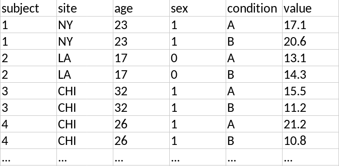
I assume that the data snippet is representative of the full dataset: every participant provides one response under each condition and that site, age and sex are participant-level covariates.
To test the hypothesis that responses are higher under A than under B, let's first estimate the condition effect: the difference between A and B adjusting for age and sex and taking into account the "subjects nested with sites" structure. So the fixed component of the linear mixed model is y ~ age + sex + condition and the random component is 1 | site/subject. This specification works "out of the box" so to say, whether there is one observation under each condition per subject or multiple — not necessarily balanced — observations per condition & subject. We just plug in the data into lme4::lmer (or nlme::lme or glmmTMB::glmmTMB or MASS::glmmPQL. For example:
m1 <- lme4::lmer(
  y ~ age + sex + condition + (1 | site/subject)
)
And if we declare the condition as factor with ordered levels c("B", "A"), with summary(m1) we get an estimate for the effect of condition A compared to that of condition B, i.e. an estimate for the difference A - B. We also get a t-statistic.
The goal of this analysis is to calculate a p-value when the alternative hypothesis is A > B. The challenge is not that the alternative is one-sided (it's easy to calculate the p-value by hand) but to determine the degrees of freedom of the t-statistic. For a linear mixed model this is not straightforward at all: getting degrees of freedom from lmer, How to determine Degrees of Freedom in Linear (Mixed Effect) Regression, Degrees freedom reported by the lmer model don't seem plausible, How to obtain the p-value (check significance) of an effect in a lme4 mixed model?. And unfortunately no agreement on the best practice emerges from those discussions either.
However, if the dataset is large enough (and the model fits the data well), the t-statistic is approximately normal. Then the choice for degrees of freedom formula doesn't make a practical difference. In a very imprecise way, by "large enough" I mean the number of subjects n is at least 50 more than the number of sites k. (Note #1: I increased this from 30 to 50; there isn't a hard-set rule anyway for when the $t$ is "sufficiently" close to the normal; see also Why does the t-distribution become more normal as sample size increases?. Note #2: We also need degrees of freedom for the covariates, so let's say n ≥ 50 + k + 2 as the age and sex covariates each have one degree of freedom.)
Finally compute the p-value for the greater-than test as:
# p-value = Pr{T < statistic}
# DF can vary depending on the method used to fit the model
pt(statistic, df, lower.tail = FALSE)

# or

# p-value = Pr{Z < statistic}  (normal approximation)
pnorm(statistic, lower.tail = FALSE)
The model y ~ age + sex + condition + (1 | site/subject) works well indeed, and since it doesn't need the data to be balanced, is probably the way to go about the analysis. Nevertheless, I also show how to estimate the difference between the two conditions with a model for the within-subject differences. This analysis has more steps and originally I had missed one of those steps — now fixed — which can be instructive. (Or at least it was instructive for me to make the mistake and then figure out how to fix it.)
First let's re-arrange the data so that each row corresponds to a subject:
#>   subject site    age   sex     A     B
#>         1 NY       23     1  17.1  20.6
#>         2 LA       17     0  13.1  14.3
#>         3 CHI      32     1  15.5  11.2
#>         4 CHI      26     1  21.2  20.8
This format highlights that the experimental design is paired as each participant provides two responses, one under A and another under B. Since the interest is whether A results in higher responses and the experimental condition varies within subject, the "basic estimators" of the difference between responses under A and B, $\Delta = \mu_A - \mu_B$, are the within-participant differences $\delta_i = Y_{i,A} - Y_{i,B}$. The hypothesis $\mu_A > \mu_B$ becomes $\Delta > 0$.
Let's add these differences to the data table:
#>   subject site    age   sex     A     B  delta
#>         1 NY       23     1  17.1  20.6 -3.5
#>         2 LA       17     0  13.1  14.3 -1.20
#>         3 CHI      32     1  15.5  11.2  4.3
#>         4 CHI      26     1  21.2  20.8  0.400
Now we can fit a mixed model for the difference between the two conditions, with covariates age and sex and a random site effect.
lmer(
  delta ~ age + sex + (1 | site)
)
In this formulation, condition doesn't appear in the model formula and the intercept term corresponds to the difference $\Delta = \mu_A - \mu_B$ when the covariates are "set to 0". However, age = 0 doesn't make sense and in any case we want an estimate of the condition effect that's representative of the entire population under study (young adults).
So we center the continuous covariate age to its mean and use the sum contrast for the categorical covariate sex. In R formula notation:
m2 <- lmer(
  delta ~ I(age - mean(age)) + sex + (1 | site),
  contrasts = list(sex = "contr.sum")
)
Note: Centering the covariates is the step I had omitted in my original answer.

