Interpolation of errors from model predictions over time-series

Question

I have a regression model:

# Create Dataset ####
# simulate exponential relationship
set.seed(123)
# generate random x values between 0 and 60
x <- runif(400, 0, 60)
y <- 1 - exp(-0.1 * x) * rnorm(400, 0.7, 0.1)

data = data.frame(sr= x, fipar = y)

# Fit a GLM model #
glm_mod <- glm(fipar ~ log(sr), data = data, family = binomial)

Let's say that I want to predict this model on new data that has been collected over time:

newdat <- data.frame(sample = c(rep('A',3),rep('B',3),rep('C',3)),
                     sr = c(1,20,55,4,11,12,2,45,20),
                     timepoint = c(1,2,3,1,2,3,1,2,3))

newpreds <- predict(glm_mod, 
                    newdata = newdat,
                    type = "response", se.fit = T)

newdat$predicted_fipar <- newpreds$fit
newdat$predicted_fipar_se <- newpreds$se.fit

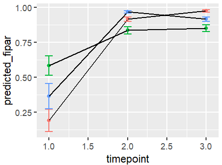
From this model, I get standard errors and can plot errorbars at the timepoint where the predictions were made, i.e

newdat %>%
  ggplot(aes(x=timepoint,y=predicted_fipar,group=sample)) +
  geom_point(aes(color=sample)) + 
  geom_line() +
  geom_errorbar(aes(ymin=predicted_fipar-predicted_fipar_se, 
                    ymax=predicted_fipar+predicted_fipar_se,
                    color=sample),
                width=0.1) 

But let's say I want to know the error at timepoint 1.5. If the interpolation between points is linear, I think that it's possible to also interpolate the error linearly (not sure if this overlooks any statistical rules), i.e:

newdat %>%
  ggplot(aes(x=timepoint,y=predicted_fipar,group=sample)) +
  geom_point(aes(color=sample)) + 
  geom_line() +
  geom_ribbon(aes(ymin=predicted_fipar-predicted_fipar_se, 
                    ymax=predicted_fipar+predicted_fipar_se,
                    fill=sample),
                alpha=0.4) +
  theme(legend.position = 'none')

But what if the interpolation between predicted points is non-linear? Are there other methods that allow this? I was thinking I should first interpolate the independent variable over time (in this case sr) and then make predictions from the model using the interpolated values. This way I can calculate the errors for the in-between points, i.e:

# Interpolate SR over time for each sample #
interpolated_sr <-
  plyr::rbind.fill(
  lapply(unique(newdat$sample),function(samp){
    sampledat <- newdat %>% 
      filter(sample == samp)
    
    sr_loess <- loess(sr ~ timepoint, data = sampledat)
    
    topred <- data.frame(sample = samp,
                         timepoint = seq(1,3,0.1))
    topred$sr <- predict(sr_loess, topred)
  
    return(topred)
    
  }))


interpolated_preds <- 
  predict(glm_mod, 
        newdata = interpolated_sr,
        type = "response", se.fit = T)

interpolated_sr$predicted_fipar <- interpolated_preds$fit
interpolated_sr$predicted_fipar_se <- interpolated_preds$se.fit

interpolated_sr %>%
  ggplot(aes(x=timepoint,y=predicted_fipar,group=sample)) +
  geom_point(aes(color=sample)) + 
  geom_line() +
  geom_ribbon(aes(ymin=predicted_fipar-predicted_fipar_se, 
                  ymax=predicted_fipar+predicted_fipar_se,
                  fill=sample),
              alpha=0.4) +
  theme(legend.position = 'none')

Is this approach valid? I understand that by interpolating the independent variable over time I am introducing some additional error from the loess model (which in this case will be very small, but could be very big depending on the fit). Is this where error propagation comes into play?

Answer 1

Your predictions and associated prediction intervals (not really errors as such) will only vary according to the value of the sr variable. So you cannot really get much sense of how these intervals will change between timepoints if you don't include sr values for any times between those timepoints. To illustrate, I below show how you can use plot_predictions() from the {marginaleffects} package to automatically compute and plot predictions and their associated uncertainties. Hopefully this makes it clear that you don't actually get any measure of uncertainty for the intervening timepoints because there is no sr value there to predict on. The plot simply draws a polygon that interpolates linearly, but this is merely a function of the plotting mechanism and not the underlying predictions:

# Simulate exponential relationship
set.seed(123)

# Generate random x values between 0 and 60
x <- runif(400, 0, 60)
y <- 1 - exp(-0.1 * x) * rnorm(400, 0.7, 0.1)

# y is a proportional variable here
hist(y)

data = data.frame(sr = x, fipar = y)

# Fit a GLM model using a Beta observation model, more appropriate
# for the proportional outcome that doesn't have a number of trials
library(mgcv)
glm_mod <- gam(fipar ~ log(sr), data = data, family = betar())

# Investigate predictions across an evenly-spaced grid of sr values
library(marginaleffects)
library(ggplot2)
plot_predictions(glm_mod, condition = 'sr') +
  theme_classic()

# Predict over the 'newdat' grid
newdat <- data.frame(sample = c(rep('A',3),
                                rep('B',3),
                                rep('C',3)),
                     sr = c(1,20,55,4,11,12,2,45,20),
                     timepoint = c(1,2,3,1,2,3,1,2,3))
plot_predictions(glm_mod, newdata = newdat, by = 'timepoint') + 
  theme_classic()

# Look at the data and you'll see that there is no prediction for the 
# intervening timepoint; the intervals you see are merely a byproduct of the
# plotting mechanism
plot_predictions(glm_mod, newdata = newdat, by = 'timepoint',
                 draw = FALSE)
#>   timepoint  estimate   std.error statistic       p.value  s.value  conf.low
#> 1         1 0.3012604 0.011258944  26.75743 1.011827e-157 521.5257 0.2791933
#> 2         2 0.9015958 0.002435880 370.13147  0.000000e+00      Inf 0.8968215
#> 3         3 0.9099221 0.002274289 400.09078  0.000000e+00      Inf 0.9054645
#>   conf.high
#> 1 0.3233276
#> 2 0.9063700
#> 3 0.9143796

^{Created on 2024-04-04 with reprex v2.1.0}