Building on Why do we need a VECM specification if the I(1) processes are cointegrated?, the error correction representation of an I(1) cointegrated system is
\begin{equation}
\Delta z_t = \alpha + \zeta_1\Delta z_{t-1} + \zeta_2\Delta z_{t-2} + \ldots + \zeta_{p-1}\Delta z_{t-p+1}+Ae_{t-1}+\epsilon_t,
\end{equation}
where $A$ contains adjustment coefficients and the $h$ rows of $B'$ are the cointegrating relationships, where $B'z_{t-1}=e_{t-1}$.
As usual, $A$ and $B'$ are not identified separately, so that, as in the example below, one typically adopts normalization restrictions such as
$$
B'=[I\quad \beta']
$$
Estimating the VAR in first differences implies omitting $Be_{t-1}$, which is relevant under cointegration.
Here is an illustration for data generated from a simple bivariate system with one cointegration relationship without lagged differences,
$$
\begin{equation}
\Delta z_t = ab'z_{t-1}+\epsilon_t.
\end{equation}
$$
Here, $z_t'=(y_t,x_t)$, $a'=(\alpha,0)$ and $b'=(1,-\beta)$.
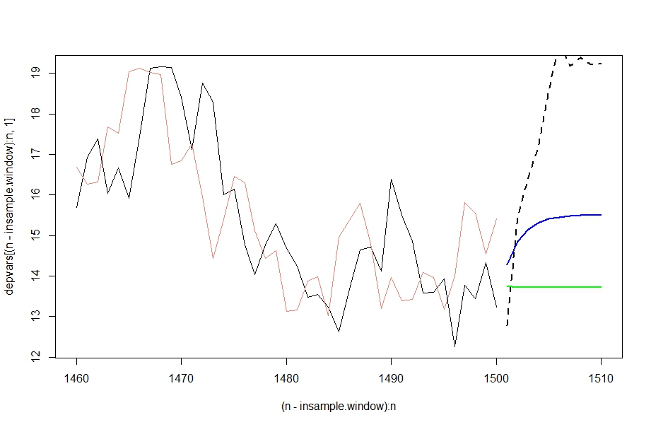
I estimate a VAR(1) for the first differences and a VECM, and report the forecasts for $y_t$ for the two models.
A representative draw is shown in the picture. In particular, the system is such that only $y_t$ adjusts to deviations from the cointegrating relationship. Here, $x_T$ (salmon) is larger than $y_T$ (black) at the end of the estimation sample. Hence, the cointegrating relationship is negative, and the negative adjustment coefficient $\alpha$ on $y_t$ implies that we expect $y_t$ to change upwards. This is also indeed what happens to $y_{T+1}, y_{T+2},\ldots$ here (dark dashed).
The VECM, and hence its forecast (blue) for $y_{T+h}$ (forecasts for $x_t$ are not shown), exploits this feature, where the VAR in differences and its forecast (green) do not. This should then lead to more accurate forecasts based on the VECM. (This is not really a foregone conclusion, though, as "misspecified", but simple models may often perform rather well in terms of prediction.)

I would suppose that these gains arise at short horizons in particular. At long horizons, one may check from the matrix $A^h$ in the code that the forecast tends to $\lim_{h\to\infty}y_{T+h}=x_T$ for the VECM while it should be close to $y_T$ (I haven't really studied this case though) for the implied VAR in levels based on the VAR estimated in first differnces, and it is not clear to me which to prefer here.
This is of course only a single illustrative run, so one should run the code many times (Monte Carlo) and compute mean MSEs over MC runs to properly assess this conjecture. For this draw, we have, from
MSE.y1.vec <- mean((depvars[(n+1):(n+oos),1]-forecasts.vec.gls)^2)
MSE.y1.var <- mean((depvars[(n+1):(n+oos),1]-forecasts.var[,1])^2)
that the VEC forecast has an MSE of about 9.28 vs. around 20.6 for the VAR in differences.
Code:
library(vars)
library(urca)
library(matrixcalc)
library(tsDyn)

n <- 1500      # a relatively large sample size to mitigate estimation error effects
oos <- 10      # prediction horizon

beta <- 1      # cointegration coeffcient on x_t
alpha <- -0.5  # only y_t error corrects here

A <- matrix(c(1+alpha, 0, -alpha*beta, 1), nrow=2) # the implied lag-1 VAR coeffcient matrix in levels
depvars <- VAR.sim(A, n+oos, include="none")       # simulate from this VAR, no deterministics for simplicity
# y <- x*beta + u.y

# implements the GLS coefficient estimator from e.g. Lütkepohl (2005), Chapter 7
# just one lag 1, no deterministics and two variables
glse.vec <- function(data){
  diffs <- diff(data)
  ls1 <- lm(diffs[,1]~head(data[,1],-1)+head(data[,2],-1)-1)
  ls2 <- lm(diffs[,2]~head(data[,1],-1)+head(data[,2],-1)-1)

  alpha <- c(coef(ls1)[1],coef(ls2)[1])
  Sigma.u <- cov(cbind(resid(ls1), resid(ls2)))

  adjusted.diffs <- diffs - head(data[,1],-1)%*%t(alpha)
  gls.tempreg1 <- lm(adjusted.diffs[,1]~head(data[,2],-1)-1)
  gls.tempreg2 <- lm(adjusted.diffs[,2]~head(data[,2],-1)-1)
  gls.adjustment <- solve(t(alpha)%*%solve(Sigma.u)%*%alpha)%*%t(alpha)%*%solve(Sigma.u)

  glse.beta <- gls.adjustment%*%c(coef(gls.tempreg1), coef(gls.tempreg2))
  return(list(alpha=alpha,beta=glse.beta))
}

estcoeffs.gls.vec <- glse.vec(depvars[1:n,])              # estimate VECM with GLS on in-sample observations

var.model <- VAR(diff(depvars[1:n,]), p = 1, type="none") # estimate VAR in first differences on in-sample observations
fc.var <- predict(var.model, n.ahead=oos)$fcst            # forecasts for first differences

# level forecast is current value plus accumulated predicted changes from VAR in first differences:
# (alternatively you can back out the implied level VAR(2) model analogously to the VECM, see appendix below)
forecasts.var <- sweep(apply(cbind(fc.var$y1[,1], fc.var$y2[,1]),2,cumsum), MARGIN = 2, cbind(depvars[n,1], depvars[n,2]), FUN = "+")

var.lvl.mat.gls <- diag(2) + estcoeffs.gls.vec$alpha%*%t(c(1, estcoeffs.gls.vec$beta))
# the level forecasts based on the implied level-VAR using the estimated VECM coefficients
# (a VAR(1) forecast w/ coefficient matrix \hat A can be written as \hat{y}_{T+h}=\hat{A}^hy_T):
forecasts.vec.gls <- sapply(1:oos, function(i) (matrix.power(var.lvl.mat.gls, i)%*%c(depvars[n,1], depvars[n,2]))[1])


insample.window <- 40
plot((n-insample.window):n, depvars[(n-insample.window):n,1], type="l", xlim=c(n-insample.window,n+oos))
lines((n-insample.window):n, depvars[(n-insample.window):n,2], col="salmon")

lines((n+1):(n+oos), depvars[(n+1):(n+oos),1], col="black", lwd=2, lty=2)
lines((n+1):(n+oos), forecasts.var[,1], col="green", lwd=2)
lines((n+1):(n+oos), forecasts.vec.gls, col="blue", lwd=2)

# the VECM-based forecast based on the true VECM coefficients at the end of the forecast horizon
matrix.power(A, oos)%*%c(depvars[n,1], depvars[n,2])

# not run
# here I tried to work with the vars and urca packages, but could not get the deterministics to be set as simply as possible
# depvars.vec <- depvars[1:n,]
# colnames(depvars.vec) <- c("y", "x")
# vec.model <- ca.jo(depvars.vec, ecdet = "none", type= "eigen", K=2)
# summary(vec.model)
# fc.vec <- predict(vec2var(vec.model, r=1), n.ahead=oos)$fcst
# forecasts.vec <- cbind(fc.vec$y[,1], fc.vec$x[,1])
# matrix.power(diag(2)+vec.model@W[,1]%*%t(vec.model@V[,1]), oos)%*%c(depvars[n,1], depvars[n,2])
# lines((n+1):(n+oos), forecasts.vec[,1], col="blue", lwd=2)

# alternative way to back out the implied VAR(2) level forecasts for the differenced model
var.coeffmat <- rbind(coef(var.model)$y1[,1],coef(var.model)$y2[,1])
(fc1 <- ((diag(2) + var.coeffmat)%*%c(depvars[n,1], depvars[n,2]) - var.coeffmat%*%c(depvars[n-1,1], depvars[n-1,2])))
forecasts.var[1,]

