Median
The cdf and pdf of continuous order statistics can be written algebraically in terms of the cdf and pdf of the original variables.
The median of an order statistic for a continuous distribution can be obtained from the median of the corresponding order statistic in the standard uniform case by transformation, noting that a continuous cdf and its inverse is a monotonic increasing (and thereby order-preserving) transformation; if half one set of values are $\leq m$ then if you transform them by a monotonic transformation $t$, half the transformed values are $\leq t(m)$.
Uniform order statistics are beta distributed, so the median of the distribution won't be in 'closed form' but it's easy enough to calculate if you can evaluate the inverse cdf of $X$.
Specifically we have:
$U_{k:n} \sim B(k,n+1-k)$
and
$U_{k:n}=F_X(X_{k:n})$.
This last equation is a fairly simple consequence of the fact that $U=F_X(X)$ is uniform. If a collection of $X_i$ values are in some order, the corresponding $U_i$ values are in that order and since $P(X_i<x)=P(U_i<F_X(x))$ the corresponding order statistics have the same relationship.
So the median of $X_{k:n}$ can be obtained by transforming that for $U_{k:n}$ by $F^{-1}$.
Casella and Berger[1] offer a proof of the cdf of an order statistic for continuous $X$ and obtain the density by differentiation (this is the one discussed in the Wikipedia page).
That the density of a uniform order statistic would be beta can be motivated readily; e.g. consider that you have a collection of independent standard uniform variates $U_1, U_2, ..., U_n$. Consider the probability that the $i$th order statistic $U_{i:n}$ is in the interval $(u,u+du)$. You need $i-1$ values to its left and $n-i$ values to its right. Which of the independent $U$'s is the one within the interval is a choice among $n$ possibilities, you need $i-1$ of the remaining $n-1$ to the left of it and the remainder to the right. So the probability of all of these events is ${{n-1}\choose{i-1}} F_U(u)^{i-1} \times (1-F_U(u))^{n-i} \times n f_U(u)$ for $0<u<1$. Now $F_U$ is just the identity in this interval and $f_U$ is $1$ in the interval, so we get: $f(u)du=n{{n-1}\choose{i-1}} u^{i-1}(1-u)^{n-i} du, \, 0<u<1$, which (dropping the $du$s) is the required density. The result for a general $X$ can either be obtained by the same form of argument (e.g. see Blitzstein & Hwang[2]), or by transformation from $U$.
Of course if you accept the density in your question as a given, we can directly write down the uniform case.
Example
Consider the fifth order statistic in a sample of size seven. We begin with the uniform. As indicated, it's distributed as a $\operatorname{Beta}(5,3)$, and so its median is (using the inverse cdf of that beta, in R):
 qbeta(.5,5,3)
[1] 0.6358839
(This is readily checked by simulation, by the way, always a good idea as it's easy to make small errors along the way.)
If you don't have a beta inverse cdf or equivalent (such as the inverse cdf for an F-distribution), then when $\min(i, n+1-i)$ is large, $\frac{i-\frac13}{n+\frac13}$ is a very good approximation to the median. Note that in our small example, finding the median exactly requires finding the real zero of a 7th degree polynomial. Even in this case, where $\min(i, n+1-i)$ is merely $3$, the approximation is fairly accurate, having a relative error of less that $0.1\%$ (the value in row 5):
> i <- 1:7
> cbind(med=qbeta(.5,i,8-i),Blom=ppoints(7,1/3))
            med       Blom
[1,] 0.09427634 0.09090909
[2,] 0.22848996 0.22727273
[3,] 0.36411609 0.36363636
[4,] 0.50000000 0.50000000
[5,] 0.63588391 0.63636364
[6,] 0.77151004 0.77272727
[7,] 0.90572366 0.90909091
Now we can directly convert to a standard Cauchy (say) from a uniform by transforming that result by the inverse cdf of the Cauchy (if you transform Cauchy variates by their cdf $F_X(X)$, you get uniforms, which we just worked out, and now we are transforming the result for the fifth-largest of them back):
> qcauchy(qbeta(.5,5,3))
[1] 0.4548645
The same strategy works for any other quantile. For example, if you wanted say the 75th percentile of the distribution of the 5th largest of 7 standard Cauchy variates:
> qcauchy(qbeta(.75,5,3))
[1] 0.9808698
Mode
Since the density of $X_{k:n}$ can be written algebraically, 'the mode' (in scare quotes because there are a number of issues that we need to address for the phrase the mode to make sense and more to readily identify it) may be doable either numerically or perhaps algebraically.
Keeping in mind the usual caveats for trying to find maxima, of course. For example, there might be multiple local modes.
The density function might not be differentiable everywhere and/or modes might not be at turning points, etc.
Note that we cannot simply use transformation from the uniform case here (quantiles are equivariant to monotonic-increasing transformations but modes are not), we must work with the density of $X_{k:n}$ directly in this case.
Let's try the same Cauchy example as before, but attempt to identify the mode instead - fortunately, in this case there is one to look for, the unique local maximum is a global maximum, it's at a turning point, and we can find it numerically. I haven't even attempted to solve it algebraically but perhaps that's doable. You might try simplifying the derivative of the density and proceed with root-finding from there, but in this case I just supplied $-\log(f)$ to an optimizer and simply used numerical derivatives:
f <- function(x) -(4*pcauchy(x,log=TRUE) + dcauchy(x,log=TRUE)
  + 2*pcauchy(x,lower.tail=FALSE,log=TRUE))
optim(1,f,method="Brent",lower=0,upper=2)
$par
[1] 0.2963231
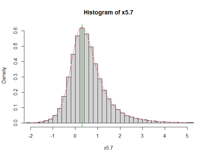
This agrees closely with the apparent location of the mode of of the density given above, and with the apparent mode of a histogram of simulated values of the given order statistic from a standard Cauchy:

It would be a relatively straightforward matter to generalize these sorts of functions, but as always with optimization (or root-finding for that matter), you must exercise a degree of care about it. Optimization is very often not nearly this neat.
[1]: Casella, George and Berger, Roger (2002), Statistical Inference (2nd ed.)
[2]: Blitzstein, Joseph K. and Hwang, Jessica (2019),
Introduction to Probability (2nd ed.)

