2
$\begingroup$

I am trying wrap my head around nested ANOVA specifically with the aov() function in R but I ran into some conceptual issues, also I believe because of inconsistencies around terminology on the internet.

As a dataset I modified a "dragons" dataset from here. Among others, now it contains a numeric response variable ("testScore"), a (nested) "lower level" factor variable ("Observer", 8 levels), and the fixed "higher level" factor variable "Species" (4 levels). The design is fairly balanced and each Species level contains two levels of Observer:

> table(dragons$Species,dragons$Observer)
           
            Erika Hannah Judith Julia Marie Paul Tarek Till
  Deathmist     0      0      0     0     0    0    55   63
  Fire          0     69      0    56     0    0     0    0
  Green         0      0      0     0    54   53     0    0
  Thorntail    64      0     66     0     0    0     0    0

The aim is to test if different levels of the predictor variable "Species" are different in the response variable "testScore", while correcting for the nesting factor "Observer".

My understanding is that a nested factor is always a type of a random effect (specifically: in which samples of a given level in the lower "random" factor always show up only in one level of the fixed "higher" factor, but fixed factor levels have samples from several random factor levels). However, ANOVAs including a "nested factor" are sometimes expressed as Y ~ A/B on the internet (having the main effect of the fixed factor A plus its interaction with the random factor B) with the terminology of "Factor B nested in fixed Factor A"...

> summary(aov(testScore~Species/Observer, data=dragons))
                  Df Sum Sq Mean Sq F value   Pr(>F)    
Species            3  12913    4304   13.30 2.38e-08 ***
Species:Observer   4  87969   21992   67.98  < 2e-16 ***
Residuals        472 152704     324 

(this results seems wrong as species whould probably not be different in testScore)

...while sometimes it is expressed as Y ~ A + Error(B/A) and the terminology switches to "fixed factor A being nested in random factor B" (see again here and the reply here)...

> summary(aov(testScore~Species+Error(Observer/Species), data=dragons))

Error: Observer
          Df Sum Sq Mean Sq F value Pr(>F)
Species    3  12913    4304   0.196  0.894
Residuals  4  87969   21992               

Error: Within
           Df Sum Sq Mean Sq F value Pr(>F)
Residuals 472 152704   323.5               
Warning message:
In aov(testScore ~ Species + Error(Observer/Species), data = dragons) :
  Error() model is singular

The latter example provides the test result I expected with Species not being different. However, the warning message raised my concerns on the validity of my model given the dataset. Also, assuming the latter approach is the correct one, when is "Y ~ A/B" used?

I would very much appreciate if somebody could help me with my confusion and maybe suggest to me what the warning message might hint at, how I can correct my model for this dataset or how the data would have to look like to work for this model. Thanks!

*** edit: here is the data on my google drive ***

$\endgroup$
8
  • $\begingroup$ I agree with @jarbet that it's better to fit a mixed model. See this note in the documentation of {stats::aov}: "aov is designed for balanced designs, and the results can be hard to interpret without balance: beware that missing values in the response(s) will likely lose the balance. If there are two or more error strata, the methods used are statistically inefficient without balance, and it may be better to use lme in package nlme." Fairly balanced is not the same as balanced. $\endgroup$
    – dipetkov
    Commented Nov 10 at 14:24
  • $\begingroup$ Why do you expect that the species are probably not different in testScore? And finally with just two observers per species, it doesn't seem reasonable to try to add a random interaction between the fixed effect (Species) and the random effect (Observer). $\endgroup$
    – dipetkov
    Commented Nov 10 at 14:39
  • $\begingroup$ Thanks for the comments. I specifically want to use the aov() function to specifically do a nested ANOVA (the internet seems to indicate that it should be possible with my data). I had already fit a mixed model using lme4, as suggested by jarbet, and all went smooth, but here it was less about getting a useful result, but about understanding why the nested ANOVA spits out the warning message and/or to understand the "correct" coding for a nested aov() model. I also attempted to fit a model with twice as many observers (see comment by dipetkov), but same warning. $\endgroup$ Commented Nov 10 at 15:06
  • $\begingroup$ lme(testScore ~ Species + (1 | Observer) -- or equivalently aov(testScore ~ Species + Error(Observer)) -- is a one-way nested ANOVA. One-way because there's one fixed effect, Species, and nested because the errors are nested within observer. I do not follow why you need more complexity in the error term. That being said, I don't know much about aov; as discussed above, mixed models are easier to fit and easier to understand. $\endgroup$
    – dipetkov
    Commented Nov 10 at 17:29
  • 1
    $\begingroup$ I edited the original question and added a link to my google drive with the csv file. Please recognize the original source of the data mentioned in the original question, which I then modified. My understanding of a crossed effect is that already one random factor can be of the crossed type, when its levels occure in all levels of the fixed effect. E.g. each of observer observed all species instead of only one. A more complex crossed design may include a random factor crossed throughout levels of another random factor, of course. Again, thank you for all the help. $\endgroup$ Commented Nov 12 at 10:43

2 Answers 2

2
$\begingroup$

Given the hierarchical structure of your data, why not try a hierarchical model such as the lme4::lmer R function? I think the code would be something like:

  • fit <- lme4::lmer(testScore ~ Species + (1 | Observer), data = dragons)

I think you can get a p-value for Species from anova(fit), if not, then load the lmerTest R package and then you can get pvalue using summary(fit).

I'm not sure the above model is the exact model you want though, but it's a start. It allows you to assess differences in mean scores between Species while accounting for different mean scores between the observers (i.e. some observers might be more likely to rate most dragons higher or most dragons lower, etc).

$\endgroup$
2
$\begingroup$

I attempt to answer only this part:

(...) suggest to me what the warning message might hint at, how I can correct my model for this dataset or how the data would have to look like to work for this model.

Discussions about terminology (nested vs crossed, fixed vs random, crossed fixed effects nested within a random effect, ...) can quickly get abstract and I'm not sure that nailing down the terminology is necessary for understanding how to model a particular experiment/dataset.

Nested ANOVA in R produces warning message "Error() model is singular"

Each observer works with one species (ie. there's no variability of Species within Observer). That's why the Error(Observer/Species) model raises a warning about singular errors.

The structure of your data indicates a one-way nested ANOVA which you can specify with

aov(Y ~ Species + Error(Observer))

"One-way" because there's one fixed effect, Species, and "nested" because the errors are grouped within the random effect, Observer.

For illustration I use the dragons dataset with some modifications. The original source of the data is this Introduction to Linear Mixed Models by the Coding Club.

I want to compare two fixed effects — one factor that varies within observer, and one factor that doesn't, so I repurpose the site variable and create a Diet variable instead, with three levels: meat, vegetarian and vegan; each data point is a different dragon and the outcome variable is body length. I also balance the dataset. (The full R code is attached at the end.)

Let's take a look at the data. The colors indicate Species, the shapes — Diet, and the panels — Observer. We can see right away that Diet varies within Observer but Species doesn't.
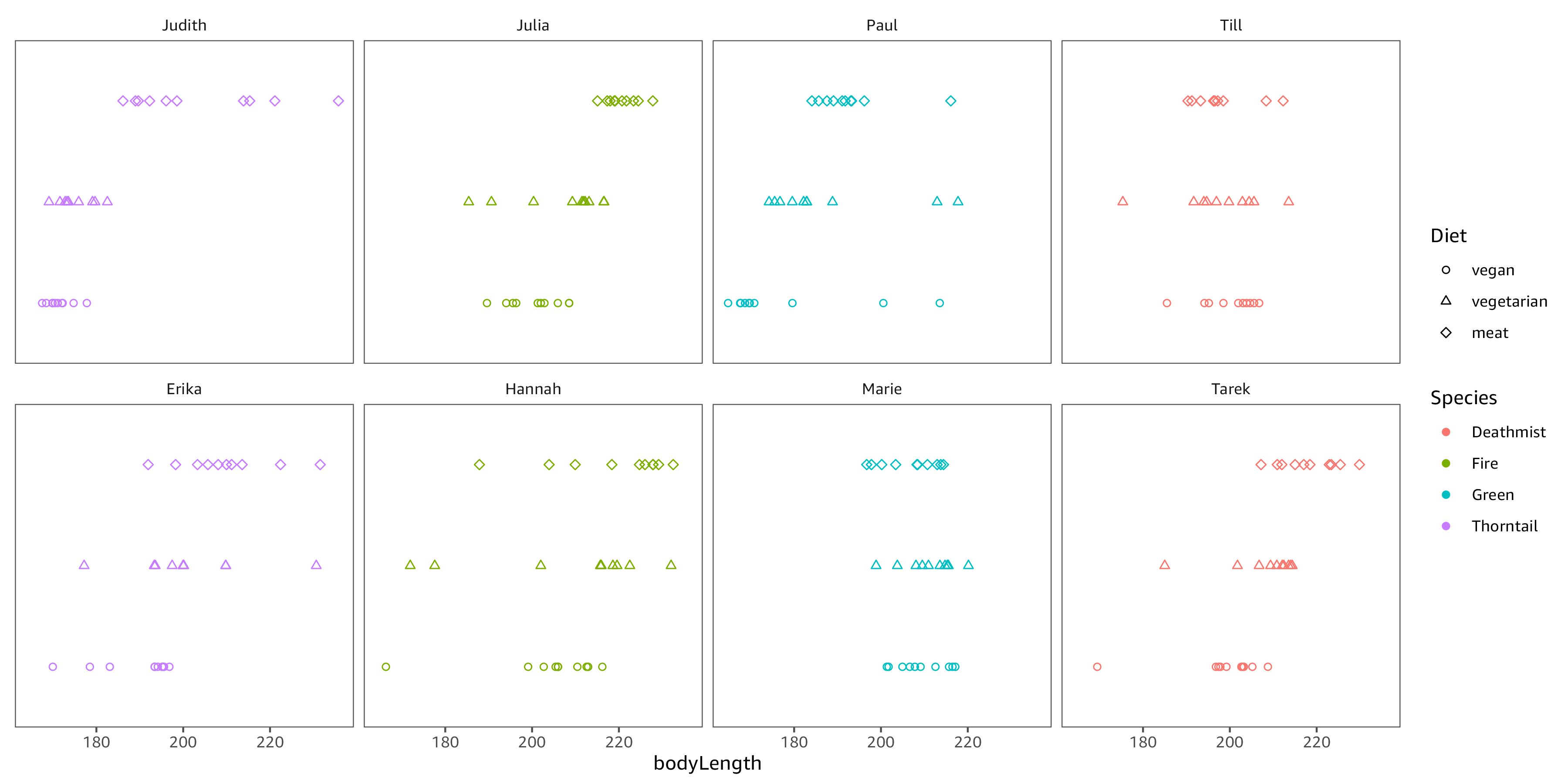
scatter plot of 2-way design

We will look at three ANOVAs. (All three models fit without warnings.)

fit1a <- aov(bodyLength ~ Species + Error(Observer), data = dragons)
fit1b <- aov(bodyLength ~ Species + Diet + Error(Observer), data = dragons)
fit1c <- aov(bodyLength ~ Species + Diet + Error(Observer / Diet), data = dragons)

The first model ignores Diet altogether.

#> aov(bodyLength ~ Species + Error(Observer), data = dragons)
#> Error: Observer
#>           Df Sum Sq Mean Sq F value Pr(>F)
#> Species    3  23146    7715   1.398  0.366
#> Residuals  4  22071    5518               
#> 
#> Error: Within
#>            Df Sum Sq Mean Sq F value Pr(>F)
#> Residuals 400  62116   155.3

The F-statistic for the Species effect is reported in the first table, Error: Observer, where the numerator degree of freedom is 3 (= #species - 1) while the denominator degrees of freedom is 4 (= #observers - #species). This is an inefficient design for estimating differences between species because we can learn about the species only from between-observer comparisons. Even though the sample size is 408, we effectively have 8 data points for the Species effect.

Now let's move to the two-way ANOVAs. These are slightly different in terms of how the within-observer factor, Diet, is modeled.

#> aov(bodyLength ~ Species + Diet + Error(Observer), data = dragons)
#> Error: Observer
#>           Df Sum Sq Mean Sq F value Pr(>F)
#> Species    3  23146    7715   1.398  0.366
#> Residuals  4  22071    5518               
#> 
#> Error: Within
#>            Df Sum Sq Mean Sq F value Pr(>F)    
#> Diet        2  14099    7049   58.43 <2e-16
#> Residuals 398  48017     121               

#> aov(bodyLength ~ Species + Diet + Error(Observer / Diet), data = dragons)
#> Error: Observer
#>           Df Sum Sq Mean Sq F value Pr(>F)
#> Species    3  23146    7715   1.398  0.366
#> Residuals  4  22071    5518               
#> 
#> Error: Observer:Diet
#>           Df Sum Sq Mean Sq F value   Pr(>F)    
#> Diet       2  14099    7049    16.2 0.000228
#> Residuals 14   6092     435                     

#> Error: Within
#>            Df Sum Sq Mean Sq F value Pr(>F)
#> Residuals 384  41925   109.2

No change as far as the Species effect is concerned (thanks to balance). The sum of squares and degrees of freedom for the Diet effect is the same as well: Sum Sq = 14,099 on 2 (= #diets - 1) degrees of freedom.

The difference is in the denominator (residual) sum of squares and degrees of freedom for the F-statistic of the Diet effect. Should we go with Error(Observer) in which case the denominator degrees of freedom are 398 = (sample size - #observers - #diets - 1)? Or should we go with Error(Observer/Diet) in which case the denominator degrees of freedom are 14 = (#observers - 1) * (#diets - 1)?

I'd say that both models could be valid and that which one is appropriate depends on how the experiment was performed. The structure of the dataset (and therefore — the terminology of "fixed" vs "crossed") doesn't give the full picture.

Say that, in preparing food for the dragons, the observers followed three specific recipes, one for each diet. Then — I think — it's appropriate to use the Error(Observer/Diet) model. As the same meat/vegetarian/vegan recipe was used throughout, we've got (pseudo?) replication for the Diet effect. We can say something about these three versions of the diets but we can say less about the benefits of meat vs vegetarian vs vegan diet in general on the body length of dragons. In this case we estimate the Diet effect from comparisons between observer × diet combinations.

Compare this with an experiment where for each dragon, the observers randomly chose the recipe on which to rear each dragon from a meat, vegetarian or vegan cook book for dragons. Now there's variability in what food dragons are raised on, even for the same observer. So the Error(Observer) model is more appropriate. In this case we estimate the Diet effect from comparisons within observers.


library("tidyverse")

dragons <-
  read_csv("dragons.csv") |>
  mutate(
    Diet = fct_recode(site, vegan = "a", vegetarian = "b", meat = "c")
  )

set.seed(1234) # for reproducibility

dragons <- dragons |>
  group_by(
    Species, Observer, Diet
  ) |>
  slice_sample(
    n = 17
  ) |>
  ungroup()

fit1a <- aov(bodyLength ~ Species + Error(Observer), data = dragons)
fit1b <- aov(bodyLength ~ Species + Diet + Error(Observer), data = dragons)
fit1c <- aov(bodyLength ~ Species + Diet + Error(Observer / Diet), data = dragons)

summary(fit1a)
summary(fit1b)
summary(fit1c)

dragons |>
  group_by(Species) |>
  mutate(
    id = dense_rank(Observer)
  ) |>
  ungroup() |>
  mutate(
    Observer = fct_reorder2(Observer, Species, id)
  ) |>
  ggplot(
    aes(bodyLength, Diet, color = Species, shape = Diet)
  ) +
  geom_point() +
  facet_wrap(
    ~Observer,
    ncol = 4
  ) +
  scale_shape_manual(
    values = c(1, 2, 5, 0, 6, 3, 4, 11)
  ) +
  theme(
    axis.title.y = element_blank(),
    axis.ticks.y = element_blank(),
    axis.text.y = element_blank(),
    strip.text.y = element_blank()
  )
$\endgroup$
1
  • $\begingroup$ In hindsight, the diet analogy might be more of a distraction than help. Seemed like good idea when I first started writing the answer. $\endgroup$
    – dipetkov
    Commented Nov 16 at 14:38

Your Answer

By clicking “Post Your Answer”, you agree to our terms of service and acknowledge you have read our privacy policy.

Not the answer you're looking for? Browse other questions tagged or ask your own question.