8
$\begingroup$

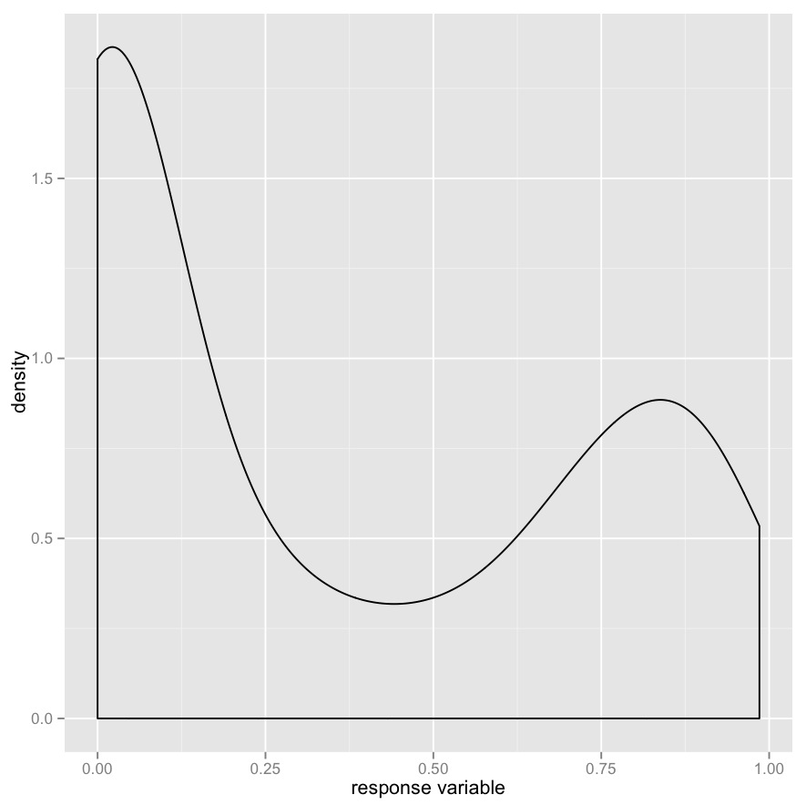
I have carried out a linear regression. The plot below shows the distribution of the response variable:

enter image description here

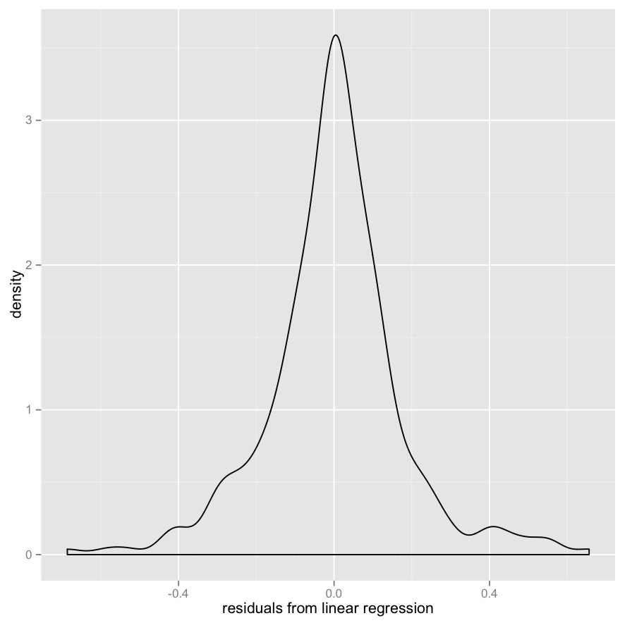
I believe the response variable is beta distributed, therefore virtually the exact opposite of normally distributed. However, when including all my predictor variables in the linear regression, the residuals turn out to be quite normally distributed, as shown in this plot:

enter image description here

Has my model satisfied the assumptions of linear regression? Might there be a better model to use?

$\endgroup$
2
  • $\begingroup$ Questions / misunderstandings about the marginal distribution of $Y$ & the distribution of $X$ are common. In addition to the good answers below, this thread: what-if-residuals-are-normally-distributed-but-y-is-not might be helpful. $\endgroup$ Commented Nov 12, 2013 at 4:33
  • $\begingroup$ Yes, what matters is distribution of errors. Distribution of y does not matter. $\endgroup$ Commented Jul 26 at 18:40

4 Answers 4

11
$\begingroup$

Your distribution is not beta if your density plot is to be taken at face value. A beta distribution cannot have two modes within (0, 1). However, no density plot for a bounded variable (at a guess here from some kernel density estimation procedure) can be taken at face value unless the estimation includes adjustments for boundary artefacts, which is not typical. But, as it were, we see what you mean.

However, to focus on the major issues:

  • A regression is first and foremost a model for the mean of a variable as it varies with the predictors. Even if an assumption of normal errors is made, that is not an assumption about the marginal distribution of the response and it is the least important assumption that is being made. So, it is not surprising that your regression behaves fairly well as far as can be inferred from the distribution of residuals if the functional form catches the way that conditional means behave.

  • The assertion of normality is more convincing if you show us a normal probability plot. That distribution looks to me to have higher kurtosis than a normal, although that is likely to be a little deal.

  • You need to check that your model is predicting values within [0,1]. Some of your residuals are about 0.7 in magnitude and so it seems possible that some of the predictions are qualitatively wrong.

  • At the same time, you should be able to do better with a regression that respects the bounded nature of the response. You could try beta regression or a generalised linear model with binomial family and logit link. The latter sounds wrong but often works well in practice. For a concise introductory review, see http://www.stata-journal.com/sjpdf.html?articlenum=st0147 Beta regression is supported in R and Stata (and likely so in other software) and generalised linear models are widely supported, although watch for routines that reject non-binary responses if a logit link is requested.

Note: The exact form of your density plot for the response is a side-issue, so I will make this an added note. It's clear that the density for a variable bounded by 0 and 1 must average 1. Your graph has a useful reference line density at 1. Visually comparing the bump above 1 on the left with the area to its right underlines that some of the density has been smoothed away by the procedure beyond the support and discarded. That is, the graph shown truncates the display: the smoothed distribution has positive density below 0 or above 1, which is not shown. There are known ways to smooth a bounded variable more respectfully, in this case including (a) to smooth logit of the variable and back-transform the density (a little problematic if observed values include 0 or 1), or (b) to reflect density inwards at the extremes. Naturally, there is scope for disagreement about whether this is trivial or secondary on the one hand or incorrect on the other. (I'd rather see a quantile plot of the data, but I'll not expand on that.)

$\endgroup$
10
$\begingroup$

The distribution of the response is irrelevant. Inference based on small samples requires the errors to be approximately normal (better look at the QQ-plot of the residuals than at its density because the tails are important). If you are only interested in descriptive results or if the sample size is not too small, you therefore do not need to worry about normality.

Much more important are the other assumptions of linear regression (correct model structure, no large outliers in the predictors and, if you are interested in inference, homoscedastic and uncorrelated errors).

$\endgroup$
2
  • 2
    $\begingroup$ Agreed on the importance of correct model structure: that is what bites and respecting the bounded character of the response is key. $\endgroup$
    – Nick Cox
    Commented Nov 2, 2013 at 11:13
  • $\begingroup$ @NickCox: we were just too busy writing answers :-) $\endgroup$
    – Michael M
    Commented Nov 2, 2013 at 11:17
2
$\begingroup$

Strictly speaking, the normality of residuals assumption is not needed for OLS to work, it becomes an issue especially in hypothesis testing. Since your residuals actually seem to be normally distributed, you're fine even in this area. Additionally, OLS does not assume anything about the distribution of variables so you do not have to worry about that.

$\endgroup$
2
$\begingroup$

Although the other answers have already addressed the question, I would like to add another powerful option that would solve most of the problems related to the distribution-assumptions: quantile regression.

Depending on the research interests, this method can be extremely powerful.

As someone has already said before, if you are merely interested in estimating the marginal mean (or any quantile) of your outcome then you don't need to worry about any assumption at all, as both quantile and ordinary regression methods perfectly estimate it.

If you are interested in inference, ordinary regression has a couple of problems with the distribution assumptions, whereas the quantile doesn't because it is distribution free. It's true that you can try using mean regression and robust estimators, but personally I prefer quantile regression, which is by the way even more informative (because you can estimate the whole conditional distribution of the outcome instead of just one of its summary indicators, the mean).

If you are interested in both prediction and inference, then the quantile's property of invariance is quite handy. For example, suppose you are working with probabilities, or rates (or any other "bounded" outcome). With quantile regression you can transform the outcome Y so that it's transformation is not bounded (for example, using a logit or probit function), model logit(Y) and use the same model for predictions and inference.

With ordinary methods it's not so easy, because of Jensen's inequality: E(g(Y)) is never equal to g(E(Y)).

Therefore, you either use two models (one for the prediction, one for the association) or you must use other methods (beta regression, logit normal regression) that, however, have problems related to respectively parameter interpretation and distribution assumptions.

Finally, there can always be problems related to the linearity assumption or independent data. In the former, we can solve the problem by adding splines (which, though, complicate the interpretation of parameters).

For the latter, instead, mixed effect regression models could help us (if we have hierarchical or longitudinal data).
$\endgroup$

Your Answer

By clicking “Post Your Answer”, you agree to our terms of service and acknowledge you have read our privacy policy.

Not the answer you're looking for? Browse other questions tagged or ask your own question.