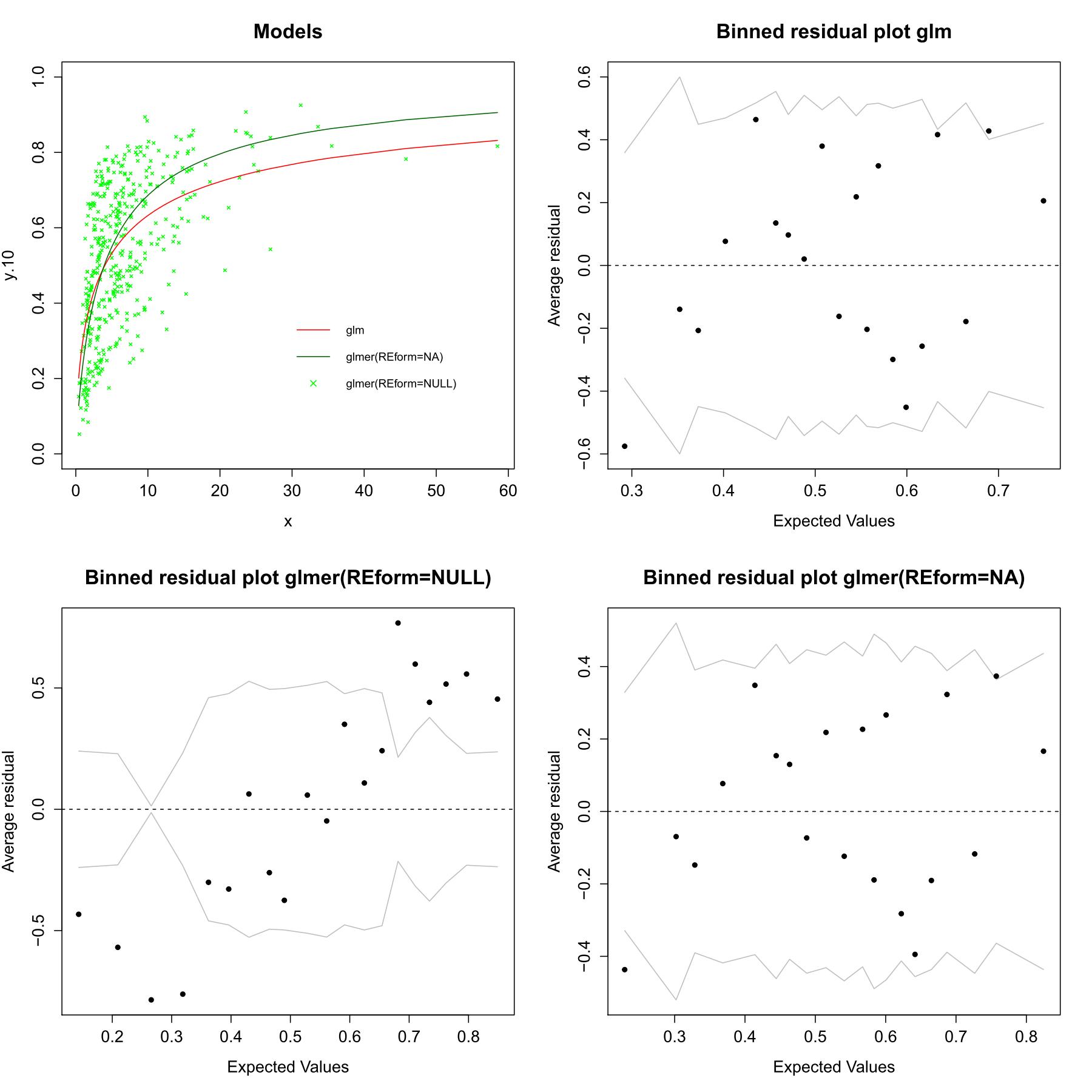
Which binnedplot of the glmer should I use to check the model? The residuals against the predicted values without random part(REform=NA) or residuals against the predicted values with random part(REform=NULL)?
I have one binary response variable (y.10) derived from one continuous variable with around 50 to 75% of zeros. I want to model the probability to exceed the limit of 10. For this example I used only one predictor "fragments" which is transformed by taking the logarithm to get a normal distribution an later a better fit . All variables are measured in tree regions (region). Within this regions are different plots (plot) and a set of samples were taken from some objects (object).
To inspect the residuals I used binnedplot like discribed in the answer of the question: Unexpected residuals plot of mixed linear model using lmer (lme4 package) in R. To save calculation time with very complex models I modeled at first with glm {stats} and based on this results the model with less variables with glmer{lme4}. Doing this I could observe a big difference in the binnedplot of residuals.
To examination the differences I created this example with only one variable. Like you can see in the picture bellow the models of glm and glmer without the random part show a very similar behavior. At the end the random part is not for interest. I need the random part only during model selection.
Which binnedplot of the glmer should I use to check the model? The residuals against the predicted values without random part(REform=NA) or residuals against the predicted values with random part(REform=NULL)?
The code and the resulting picture is given here:
fit.glm=glm(y.10 ~ x.t , data=data, family="binomial")
fit.glmer=glmer(y.10 ~ x.t + (1|region) + (1|plot) + (1|object),
          data=data, family="binomial")

y.glm=predict(fit.glm, type ="response")
y.glmer=predict(fit.glmer,REform=NA,type ="response")
y.glmer.ran=predict(fit.glmer,REform=NULL,type ="response")

par(mfrow=c(2,2))
plot(y.10~x, data=data, type="n", main="Models")
points(y.glmer.ran~data$x, col="green", pch=4, cex=0.5)
lines(y.glm~data$x, col="red")
lines(y.glmer~data$x, col="darkgreen")

binnedplot(fitted(fit.glm),resid(fit.glm), main="Binned residual plot glm")
binnedplot(y.glmer.ran,resid(fit.glmer), main="Binned residual plot glmer(REform=NULL)")
binnedplot(y.glmer,resid(fit.glmer), main="Binned residual plot glmer(REform=NA)")

