Expected number of ratio of girls vs boys birth

Question

I have came across a question in job interview aptitude test for critical thinking. It is goes something like this:

The Zorganian Republic has some very strange customs. Couples only wish to have female children as only females can inherit the family's wealth, so if they have a male child they keep having more children until they have a girl. If they have a girl, they stop having children. What is the ratio of girls to boys in Zorgania?

I don't agree with the model answer given by the question writer, which is about 1:1. The justification was any birth will always have a 50% chance of being male or female.

Can you convince me with a more mathematical vigorous answer of $\text{E}[G]:\text{E}[B]$ if $G$ is the number of girls and B is the number of boys in the country?

Answer 1

Start with no children

repeat step

{

Every couple who is still having children has a child. Half the couples have males and half the couples have females.

Those couples that have females stop having children

}

At each step you get an even number of males and females and the number of couples having children reduces by half (ie those that had females won't have any children in the next step)

So, at any given time you have an equal number of males and females and from step to step the number of couples having children is falling by half. As more couples are created the same situation reoccurs and all other things being equal, the population will contain the same number of male and females

Answer 2

Let $X$ be the number of boys in a family. As soon as they have a girl, they stop, so

\begin{array}{| l |l | } \hline X=0 & \text{if the first child was a girl}\\ X=1 & \text{if the first child was a boy and the second was a girl}\\ X=2 & \text{if the first two children were boys and the third was a girl}\\ \text{and so on}\ldots &\\ \hline \end{array}

If $p$ is the probability that a child is a boy and if genders are independent between children, the probability that a family ends up having $k$ boys is $$\mbox{P}(X=k)=p^{k}\cdot (1-p),$$ i.e. the probability of having $k$ boys and then having a girl. The expected number of boys is $$ \operatorname{E}X=\sum_{k=0}^\infty kp^k \cdot (1-p)=\sum_{k=0}^\infty kp^k-\sum_{k=0}^\infty kp^{k+1}.$$ Noting that $$\sum_{k=0}^\infty kp^k=\sum_{k=0}^\infty (k+1)p^{k+1}$$ we get $$\sum_{k=0}^\infty kp^k-\sum_{k=0}^\infty kp^{k+1}=\sum_{k=0}^\infty (k+1)p^{k+1}-\sum_{k=0}^\infty kp^{k+1}=\sum_{k=0}^\infty p^{k+1}=p\sum_{k=0}^\infty p^{k}=\frac{p}{1-p}$$ where we used that $\sum_{k=0}^\infty p^k=1/(1-p)$ when $0<p<1$ (see geometric series).

If $p=1/2$, we have that $\operatorname{E}X=0.5/0.5$. That is, the average family has 1 boy. We already know that all families have 1 girl, so the ratio will over time even out to be $1/1=1$.

The random variable $X$ is known as a geometric random variable.

Answer 3

Summary

The simple model that all births independently have a 50% chance of being girls is unrealistic and, as it turns out, exceptional. As soon as we consider the consequences of variation in outcomes among the population, the answer is that the girl:boy ratio can be any value not exceeding 1:1. (In reality it likely still would be close to 1:1, but that's a matter for data analysis to determine.)

Because these two conflicting answers are both obtained by assuming statistical independence of birth outcomes, an appeal to independence is an insufficient explanation. Thus it appears that variation (in the chances of female births) is the key idea behind the paradox.

Introduction

A paradox occurs when we think we have good reasons to believe something but are confronted with a solid-looking argument to the contrary.

A satisfactory resolution to a paradox helps us understand both what was right and what may have been wrong about both arguments. As is often the case in probability and statistics, both arguments can actually be valid: the resolution will hinge on differences among assumptions that are implicitly made. Comparing these different assumptions can help us identify which aspects of the situation lead to different answers. Identifying these aspects, I maintain, is what we should value the most.

Assumptions

As evidenced by all the answers posted so far, it is natural to assume that female births occur independently and with constant probabilities of $1/2$. It is well known that neither assumption is actually true, but it would seem that slight deviations from these assumptions should not affect the answer much. Let us see. To this end, consider the following more general and more realistic model:

1. In each family $i$ the probability of a female birth is a constant $p_i$, regardless of birth order.

2. In the absence of any stopping rule, the expected number of female births in the population should be close to the expected number of male births.

3. All birth outcomes are (statistically) independent.

This is still not a fully realistic model of human births, in which the $p_i$ may vary with the age of the parents (particularly the mother). However, it is sufficiently realistic and flexible to provide a satisfactory resolution of the paradox that will apply even to more general models.

Analysis

Although it is interesting to conduct a thorough analysis of this model, the main points become apparent even when a specific, simple (but somewhat extreme) version is considered. Suppose the population has $2N$ families. In half of these the chance of a female birth is $2/3$ and in the other half the chance of a female birth is $1/3$. This clearly satisfies condition (2): the expected numbers of female and male births are the same.

Consider those first $N$ families. Let us reason in terms of expectations, understanding that actual outcomes will be random and therefore will vary a little from the expectations. (The idea behind the following analysis was conveyed more briefly and simply in the original answer which appears at the very end of this post.)

Let $f(N,p)$ be the expected number of female births in a population of $N$ with constant female birth probability $p$. Obviously this is proportional to $N$ and so can be written $f(N,p) = f(p)N$. Similarly, let $m(p)N$ be the expected number of male births.

• The first $pN$ families produce a girl and stop. The other $(1-p)N$ families produce a boy and continue bearing children. That's $pN$ girls and $(1-p)N$ boys so far.

• The remaining $(1-p)N$ families are in the same position as before: the independence assumption (3) implies that what they experience in the future is not affected by the fact their firstborn was a son. Thus, these families will produce $f(p)[(1-p)N]$ more girls and $m(p)[(1-p)N]$ more boys.

Adding up the total girls and total boys and comparing to their assumed values of $f(p)N$ and $m(p)N$ gives equations

$$f(p)N = pN + f(p)(1-p)N\ \text{ and }\ m(p)N = (1-p)N + m(p)(1-p)N$$

with solutions

$$f(p) = 1\ \text{ and }\ m(p) = \frac{1}{p}-1.$$

The expected number of girls in the first $N$ families, with $p=2/3$, therefore is $f(2/3)N = N$ and the expected number of boys is $m(2/3)N = N/2$.

The expected number of girls in the second $N$ families, with $p=1/3$, therefore is $f(1/3)N = N$ and the expected number of boys is $m(1/3)N = 2N$.

The totals are $(1+1)N = 2N$ girls and $(1/2+2)N = (5/2)N$ boys. For large $N$ the expected ratio will be close to the ratio of the expectations,

$$\mathbb{E}\left(\frac{\text{# girls}}{\text{# boys}}\right) \approx \frac{2N}{(5/2)N} = \frac{4}{5}.$$

The stopping rule favors boys!

More generally, with half the families bearing girls independently with probability $p$ and the other half bearing boys independently with probability $1-p$, conditions (1) through (3) continue to apply and the expected ratio for large $N$ approaches

$$\frac{2p(1-p)}{1 - 2p(1-p)}.$$

Depending on $p$, which of course lies between $0$ and $1$, this value can be anywhere between $0$ and $1$ (but never any larger than $1$). It attains its maximum of $1$ only when $p=1/2$. In other words, an expected girl:boy ratio of 1:1 is a special exception to the more general and realistic rule that stopping with the first girl favors more boys in the population.

Resolution

If your intuition is that stopping with the first girl ought to produce more boys in the population, then you are correct, as this example shows. In order to be correct all you need is that the probability of giving birth to a girl varies (even by just a little) among the families.

The "official" answer, that the ratio should be close to 1:1, requires several unrealistic assumptions and is sensitive to them: it supposes there can be no variation among families and all births must be independent.

Comments

The key idea highlighted by this analysis is that variation within the population has important consequences. Independence of births--although it is a simplifying assumption used for every analysis in this thread--does not resolve the paradox, because (depending on the other assumptions) it is consistent both with the official answer and its opposite.

Note, however, that for the expected ratio to depart substantially from 1:1, we need a lot of variation among the $p_i$ in the population. If all the $p_i$ are, say, between 0.45 and 0.55, then the effects of this variation will not be very noticeable. Addressing this question of what the $p_i$ really are in a human population requires a fairly large and accurate dataset. One might use a generalized linear mixed model and test for overdispersion.

If we replace gender by some other genetic expression, then we obtain a simple statistical explanation of natural selection: a rule that differentially limits the number of offspring based on their genetic makeup can systematically alter the proportions of those genes in the next generation. When the gene is not sex-linked, even a small effect will be multiplicatively propagated through successive generations and can rapidly become greatly magnified.

---

Original answer

Each child has a birth order: firstborn, second born, and so on.

Assuming equal probabilities of male and female births and no correlations among the genders, the Weak Law of Large Numbers asserts there will be close to a 1:1 ratio of firstborn females to males. For the same reason there will be close to a 1:1 ratio of second born females to males, and so on. Because these ratios are constantly 1:1, the overall ratio must be 1:1 as well, regardless of what the relative frequencies of birth orders turn out to be in the population.

Answer 4

The birth of each child is an independent event with P=0.5 for a boy and P=0.5 for a girl. The other details (such as the family decisions) only distract you from this fact. The answer, then, is that the ratio is 1:1.

To expound on this: imagine that instead of having children, you're flipping a fair coin (P(heads)=0.5) until you get a "heads". Let's say Family A flips the coin and gets the sequence of [tails, tails, heads]. Then Family B flips the coin and gets a tails. Now, what's the probability that the next will be heads? Still 0.5, because that's what independent means. If you were to do this with 1000 families (which means 1000 heads came up), the expected total number of tails is 1000, because each flip (event) was completely independent.

Some things are not independent, such as the sequence within a family: the probability of the sequence [heads, heads] is 0, not equal to [tails, tails] (0.25). But since the question isn't asking about this, it's irrelevant.

Answer 5

Imagine tossing a fair coin until you observe a head. How many tails do you toss?

$P(0 \text{ tails}) = \frac{1}{2}, P(1 \text{ tail}) = (\frac{1}{2})^2, P(2 \text{ tails}) = (\frac{1}{2})^3, ...$

The expected number of tails is easily calculated* to be 1.

The number of heads is always 1.

* if this is not clear to you, see 'outline of proof' here

Answer 6

Couples with exactly one girl and no boys are the most common

The reason this all works out is because the probability of the one scenario in which there are more girls is much larger than the scenarios where there are more boys. And the scenarios where there are lots more boys have very low probabilities. The specific way it works itself out is illustrated below

NumberOfChilden Probability  Girls   Boys  
1               0.5           1       0  
2               0.25          1       1  
3               0.125         1       2  
4               0.0625        1       3  
...             ...           ...     ...  

NumberOfChilden Probability   Girls*probabilty   Boys*probabilty 
1               0.5           0.5                0
2               0.25          0.25               0.25
3               0.125         0.125              0.25
4               0.0625        0.0625             0.1875
5               0.03125       0.03125            0.125
...             ...           ...                ...  
n               1/2^n         1/(2^n)            (n-1)/(2^n)

You can pretty much see where this is going at this point, the total of the girls and boys are both going to add up to one.

Expected girls from one couple${}=\sum_{n=1}^\infty(\frac{1}{2^n})=1 $
Expected boys from one couple${}=\sum_{n=1}^\infty(\frac{n-1}{n^2})=1 $

^{Limit solutions from wolfram}

Any birth, whatever family is it in has a 50:50 chance of being a boy or a girl

This all makes intrinsic sense because (try as couples might) you can't control the probability of a specific birth being a boy or a girl. It doesn't matter whether a child is born to a couple with no children or a family of a hundred boys; the chance is 50:50 so if each individual birth has a 50:50 chance then you should always get half boys and half girls. And it doesn't matter how you shuffle the births between families; you're not going to affect that.

This works for any¹ rule

For due to the 50:50 chance for any birth the ratio will end up as 1:1 for any (reasonable¹) rule you can come up with. For example the similar rule below also works out even

Couples stop having children when they have a girl, or have two children

NumberOfChilden Probability   Girls   Boys
1               0.5           1       0
2               0.25          1       1
2               0.25          0       2

In this case the total expected children is more easily calculated

Expected girls from one couple${}=0.5\cdot1 + 0.25\cdot1 =0.75$
Expected boys from one couple${}=0.25\cdot1 + 0.25\cdot2 =0.75$

¹As I said this works for any reasonable rule that could exist in the real world. An unreasonable rule would be one in which the expected children per couple was infinite. For example "Parents only stop having children when they have twice as many boys as girls", we can use the same techniques as above to show that this rule gives infinite children:

NumberOfChilden Probability   Girls   Boys
3               0.125         1       2
6               1/64          2       4
9               1/512         3       6
3*m             1/((3m)^2     m       2m

We can then find the number of parents with a finite number of children

Expected number of parents with finite children${}=\sum_{m=1}^\infty(\frac{1}{1/(3m)^2})=\frac{\pi^2}{54}=0.18277\ldots. $

^{Limit solutions from wolfram}

So from that we can establish that 82% of parents would have an infinite number of children; from a town planning point of view this would probably cause difficulties and shows that this condition couldn't exist in the real world.

Answer 7

You can also use simulation:

p<-0
for (i in 1:10000){
  a<-0
  while(a != 1){   #Stops when having a girl
    a<-as.numeric(rbinom(1, 1, 0.5))   #Simulation of a new birth with probability 0.5
    p=p+1   #Number of births
  }
}
(p-10000)/10000   #Ratio

Answer 8

Mapping this out helped me better see how the ratio of the birth population (assumed to be 1:1) and the ratio of the population of children would both be 1:1. While some families would have multiple boys but only one girl, which initially led me to think there would be more boys than girls, the number of those families would not be greater than 50% and would diminish by half with each additional child, while the number of one-girl-only families would be 50%. The number of boys and girls would thus balance each other out. See the totals of 175 at the bottom.

Answer 9

What you got was the simplest, and a correct answer. If the probability of a newborn child being a boy is p, and children of the wrong gender are not met by unfortunate accidents, then it doesn't matter if the parents make decisions about having more children based on the gender of the child. If the number of children is N and N is large, you can expect about p * N boys. There is no need for a more complicated calculation.

There are certainly other questions, like "what is the probability that the youngest child of a family with children is a boy", or "what is the probability that the oldest child of a family with children is a boy". (One of these has a simple correct answer, the other has a simple wrong answer and getting a correct answer is tricky).

Answer 10

Let

$\text{$\Omega$={(G),(B,G),(B,B,G),$\dots$}}$

be the sample space and let

$\text{X: $\Omega\longrightarrow\mathbb{R}$; $\omega\mapsto\vert\omega\vert$-1}$

be the random variable that maps each outcome, $\omega$, onto the number of boys it involves. The expected value of boys, $\text{E(X)}$, comes then down to

$\text{E(X)=$\sum_{n=1}^\infty(\text{n-1})\cdot0.5^n$=1}$,

Trivially, the expected value of girls is 1. So the ratio is 1, too.

Answer 11

It's a trick question. The ratio stays the same (1:1). The right answer is that it does not affect birth ratio, but it does affect the number of children per family with a limiting factor of an average of 2 births per family.

This is the kind of question you might find on a logic test. The answer is not about birth ratio. That's a distraction.

This is not a probability question, but a cognitive reasoning question. Even if you answered 1:1 ratio, you still failed the test.

Answer 12

I am showing the code I wrote for a Monte Carlo simulation (500x1000 families) using `MATLAB' software. Please scrutinise the code so that I did not make a mistake.

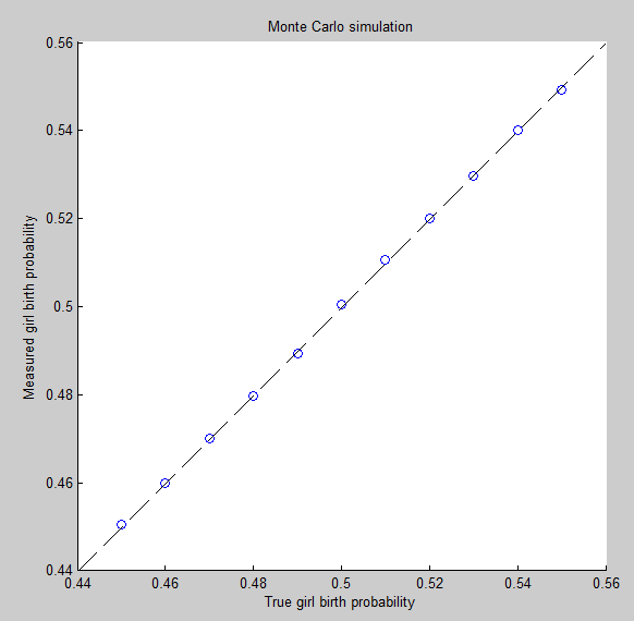
The result is generated and plotted below. It shows the simulated girl birth probability has very good agreement with the underlying natural birth probability regardless of the stopping rule for a range of natural birth probability.

Playing around with the code it is easier to understand one point I didn't quite do before---as other's point out, the stopping rule is a distraction. The stopping rule only affects the number of families given a fixed population, or from another point of view the number of child births given a fixed number of families. The gender is solely determined by dice roll and hence the ratio or probability (which is independent of number of children) will solely depend on the natural boy:girl birth rato.

testRange=0.45:0.01:0.55;
N=uint32(100000); %Used to approximate probability distribution
M=1000; %Number of families
L=500; %Monte Carlo repetitions
Nfamily=zeros(length(testRange),1);
boys=zeros(length(testRange),1);
girls=zeros(length(testRange),1);
for l = 1:L
    j=1; %Index variable for the different bgratio
    for bgratio=testRange
    k=1; %Index variable for family in each run (temp family id)
    vec=zeros(N,1);
    vec(1:N*bgratio,1)=1; %Approximate boy:girl population for dice roll, 
    %1 = boy

    vec=vec(randperm(s,N)); %Random permutation, technically not necessary 
    %due to randi used later, just be safe
    bog = vec(randi(N)); %boy or girl? (God's dice roll)

    while k<M %For M families...
        if bog == 1 %if boy:
            boys(j) = boys(j)+1; %total global boys tally
        else
            girls(j)=girls(j)+1; %total global girls tally
            %Family stops bearing children
            Nfamily(j) = Nfamily(j)+1; %total global family tally
            k=k+1; %temp family id
            %Next family...
        end
        bog=vec(randi(N)); %Sample next gender (God's dice roll)
    end

    j=j+1; %Index variable for the different bgratio
    end
end
figure;
scatter(testRange,girls./(boys+girls))
hold on
line([0 1],[0 1],'LineStyle','--','Color','k')
axis([0.44 0.56 0.44 0.56])

Answer 13

Let the random variable denoting the $i^{th}$ child in the country be $X_i$ taking on values 1 and 0 if the child is a boy or girl respectively. Assume that the marginal probability that each birth is a boy or girl is $0.5$.

The expected number of boys in the country = $E[\sum_i X_i] = \sum_i E[X_i] = 0.5 n$ (where $n$ is the number of children in the country.)

Similarly the expected number of girls = $E[\sum_i (1- X_i)] = \sum_i E[1-X_i] = 0.5 n$.

The independence of the births is irrelevant for the calculation of expected values.

---

Apropos @whuber's answer, if there is a variation of the marginal probability across families, the ratio becomes skewed towards boys, due to there being more children in families with higher probability of boys than families with a lower probability, thereby having an augmentative effect of the expected value sum for the boys.

Answer 14

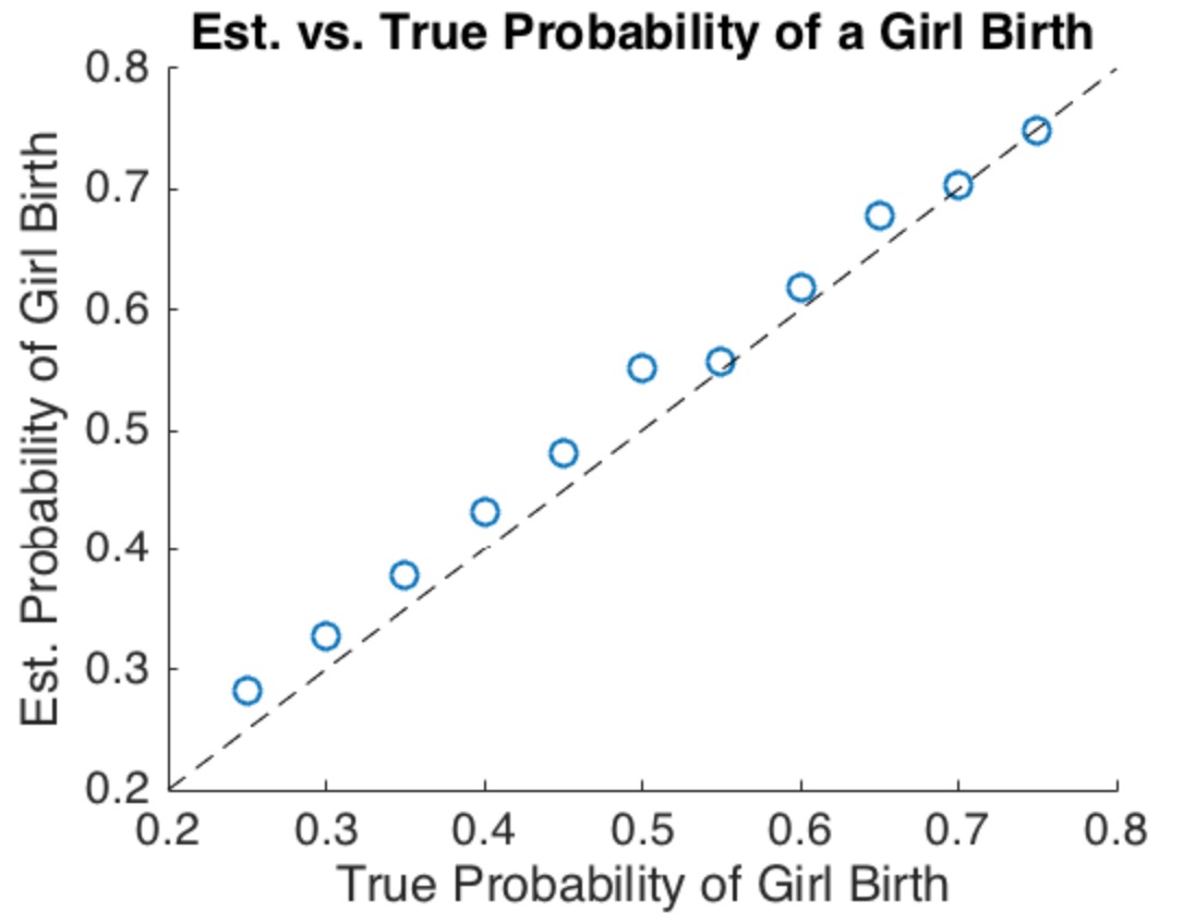
I independently also programmed a simulation in matlab, prior to seeing what others have done. Strictly speaking it is not a MC because I only run the experiment once. But once is sufficient to obtain results. Here is what my simulation yields. I don't take a stand on the probability of births being p=0.5 as a primitive. I let the birth probability vary over a range of Pr(Boys=1)=0.25:0.05:0.75.

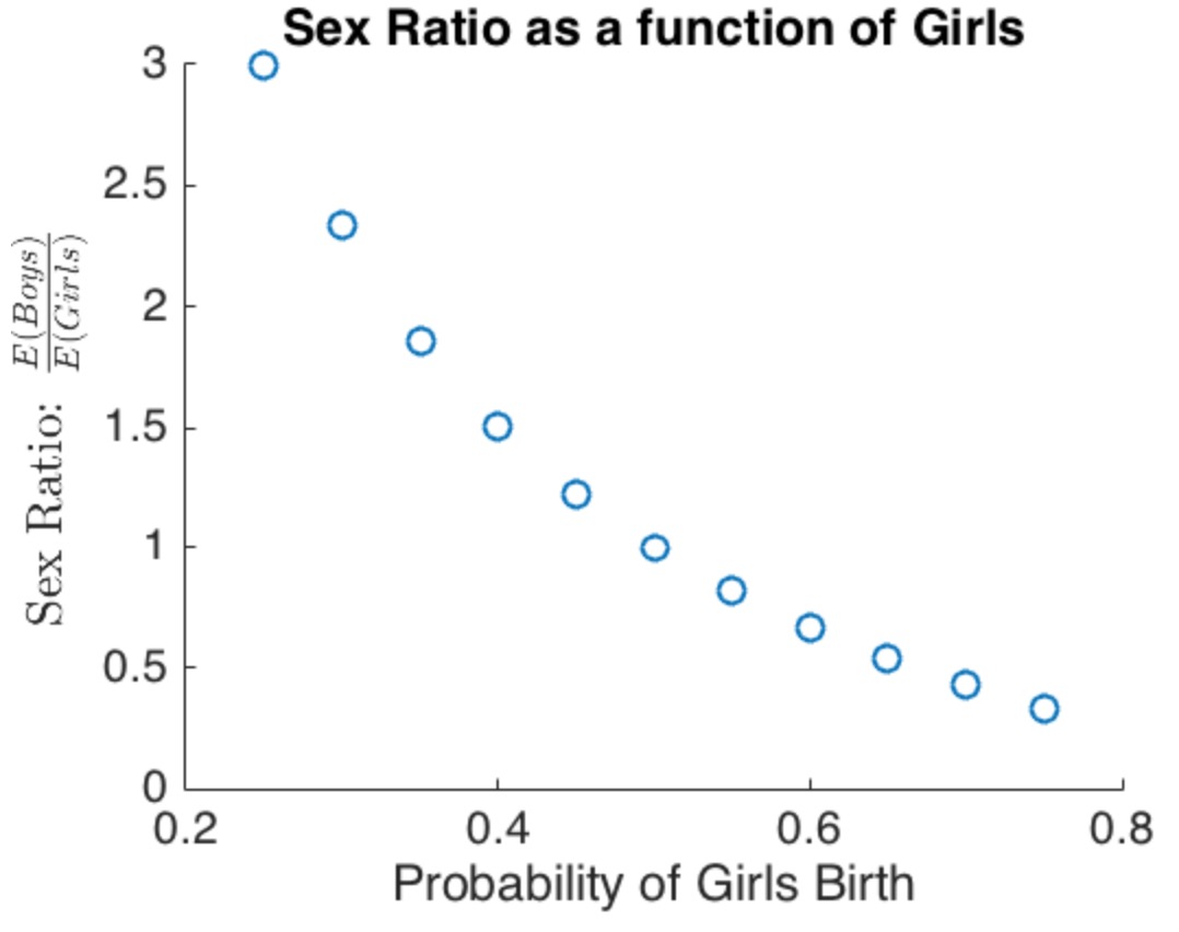
My results show that as the probability deviates from p=0.5, the sex ratio is different from 1: in expectation the sex ratio is simply the ratio of the probability of a boy's birth to the probability of a girl's birth. That is, this is a geometric random variable as identified previously by @månst. This is what I believe the original poster was intuiting.

My results closely mimic what the above poster with the matlab code has done, matching the sex ratios at the 0.45, 0.50, and 0.55 probabilities that a boy is born. I present mine as I take a slightly different approach to get at the results with faster code. To accomplish the comparison I omitted the code section vec=vec(randperm(s,N)) since s is not defined in their code and I don't know the original intention of this variable (this code section also seems superfluous - as originally stated).

I post my code

clear all; rng('default')

prob_of_boy = 0.25:0.05:0.75;
prob_of_girls = 1 - prob_of_boy;

iterations = 200;

sex_ratio = zeros(length(prob_of_boy),1);
prob_of_girl_est = zeros(length(prob_of_boy),1);
rounds_of_reproduction = zeros(length(prob_of_boy),1);

for p=1:length(prob_of_boy)

    pop = 1000000;

    boys = zeros(iterations,1);
    girls = zeros(iterations,1);
    prob_of_girl = zeros(iterations,1);

    for i=1:iterations

        x = rand(pop,1);
        x(x<prob_of_boy(p))=1;

        %count the number of boys and girls
        num_boys = sum(x(x==1));

        boys(i) = num_boys;
        girls(i) = pop - num_boys;

        prob_of_girl(i) = girls(i)/(pop);

        %Only families that had a boy continue to reproduce
        x = x(x==1);

        %new population of reproducing parents
        pop = length(x);

        %check that there are no more boys 
        if num_boys==0

            boys(i+1:end)=[];
            girls(i+1:end)=[];
            prob_of_girl(i+1:end)=[];
            break

        end
    end

    prob_of_girl_est(p) = mean(prob_of_girl(prob_of_girl~=0));
    sex_ratio(p) = sum(boys)/sum(girls);
    rounds_of_reproduction(p) = length(boys);
end

scatter(prob_of_girls,prob_of_girl_est)
hold on
title('Est. vs. True Probability of a Girl Birth')
ylabel('Est. Probability of Girl Birth')
xlabel('True Probability of Girl Birth')
line([0 1],[0 1],'LineStyle','--','Color','k')
axis([0.2 0.8 0.2 0.8])

scatter(prob_of_girls,sex_ratio)
hold on
title('Sex Ratio as a function of Girls')
xlabel('Probability of Girls Birth')
ylabel('Sex Ratio: $\frac{E(Boys)}{E(Girls)}$','interpreter','latex')

scatter(prob_of_girls,rounds_of_reproduction)
hold on
title('Rounds of Reproduction a function of Girls')
xlabel('Probability of Girls Birth')
ylabel('Rounds of Reproduction')

The following graph is expected given the strong law of large number. I reproduce it, but the graph that matters is the second graph.

Here, a population probability other than 0.5 for the birth of either sex of a child will alter the sex ratio in the overall population. Assuming that births are independent (but not the choice to keep reproducing), in each round of conditional reproduction the population probability governs the overall make up of the outcomes of boy and girl births. So as others have mentioned, the stopping rule in the problem is inconsequential to the population outcome, as answered by the poster who identified this as the geometric distribution.

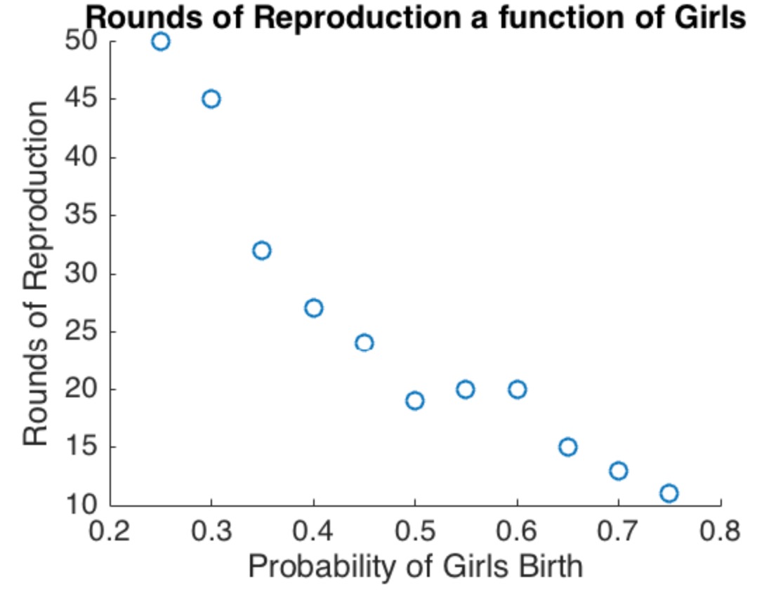
For completeness, what the stopping rule does affect is the number of rounds of reproduction in the population. Since I only run the experiment once, the graph is a bit jagged. But the intuition is there: for a given population size, as the probability of a girl's birth increases we see that families need less rounds of reproduction to obtain their desired girl before the entire population stops reproducing (obviously the number of rounds will depend on the population size, since it mechanistically increases the likelihood that a family will have, for example, 49 boys before they get their first girl)

The comparison between my calculated sex ratios:

[sex_ratio' prob_of_boy']

0.3327    0.2500
0.4289    0.3000
0.5385    0.3500
0.6673    0.4000
0.8186    0.4500
1.0008    0.5000
1.2224    0.5500
1.5016    0.6000
1.8574    0.6500
2.3319    0.7000
2.9995    0.7500

and those from the previous poster with the matlab code:

[boys./girls testRange']

0.8199    0.4500
0.8494    0.4600
0.8871    0.4700
0.9257    0.4800
0.9590    0.4900
1.0016    0.5000
1.0374    0.5100
1.0836    0.5200
1.1273    0.5300
1.1750    0.5400
1.2215    0.5500

They are equivalent results.

Answer 15

It depends on the number of families.

Let $X$ be the number of children in a family, it is geometric random variable with $p=0.5$, i.e., $$ P(X = x) = 0.5^x, x=1,2,3... $$ which implies $E(X) = 2$

Suppose there are $N$ families in the country, the girl ratio is $$ \frac{N}{ \sum X_i} $$

Since $\sum X_i /N \rightarrow E(X) = 2$ (law of large number), the ratio coverages to 1/2 if $N \rightarrow \infty$.

If there are only finite families, let $T$ be the total number of children of the country: $T = \sum X_i$, then $T$ has a negative binomial distribution with pmf $$ P(T=t) = C^{t-1}_{N-1} 0.5^t, t = N, N+1... $$

It implies $$ E\left[ \frac{N}{\sum X_i} \right] = E\left[ \frac{N}{T} \right] = \sum_{t=N}^{\infty} \frac{N}{t} C^{t-1}_{N-1} 0.5^t = {_2F_1} (N, 1, N+1, -1) $$ where $_2F_1$ is the hypergeometric function.

Therefore the expected girl ratio is ${_2F_1} (N, 1, N+1, -1) $.