Practically speaking, how do people handle ANOVA when the data doesn't quite meet assumptions?

Question

This isn't a strictly stats question--I can read all the textbooks about ANOVA assumptions--I'm trying to figure out how actual working analysts handle data that doesn't quite meet the assumptions. I've gone through a lot of questions on this site looking for answers and I keep finding posts about when not to use ANOVA (in an abstract, idealized mathematical context) or how to do some of the things I describe below in R. I'm really trying to figure out what decisions people actually make and why.

I'm running analysis on grouped data from trees (actual trees, not statistical trees) in four groups. I've got data for about 35 attributes for each tree and I'm going through each attribute to determine if the groups differ significantly on that attribute. However, in a couple of cases, the ANOVA assumptions are slightly violated because the variances aren't equal (according to a Levene's test, using alpha=.05).

As I see it, my options are to: 1. Power transform the data and see if it changes the Levene p-val. 2. Use a non-parametric test like a Wilcoxon (if so, which one?). 3. Do some kind of correction to the ANOVA result, like a Bonferroni (I'm not actually sure if something like this exists?). I've tried the first two options and gotten slightly different results--in some cases one approach is significant and the other is not. I'm afraid of falling into the p-value fishing trap, and I'm looking for advice that will help me justify which approach to use.

I've also read some things that suggest that heteroscedasticity isn't really that big of a problem for ANOVA unless the means and variances are correlated (i.e. they both increase together), so perhaps I can just ignore the Levene's result unless I see a pattern like that? If so, is there a test for this?

Finally, I should add that I'm doing this analysis for publication in a peer-reviewed journal, so whatever approach I settle on has to pass muster with reviewers. So, if anyone can provide links to similar, published examples that would be fantastic.

Answer 1

I'm trying to figure out how actual working analysts handle data that doesn't quite meet the assumptions.

It depends on my needs, which assumptions are violated, in what way, how badly, how much that affects the inference, and sometimes on the sample size.

I'm running analysis on grouped data from trees in four groups. I've got data for about 35 attributes for each tree and I'm going through each attribute to determine if the groups differ significantly on that attribute. However, in a couple of cases, the ANOVA assumptions are slightly violated because the variances aren't equal (according to a Levene's test, using alpha=.05).

1) If sample sizes are equal, you don't have much of a problem. ANOVA is quite (level-)robust to different variances if the n's are equal.

2) testing equality of variance before deciding whether to assume it is recommended against by a number of studies. If you're in any real doubt that they'll be close to equal, it's better to simply assume they're unequal.

Some references:

Zimmerman, D.W. (2004),
"A note on preliminary tests of equality of variances."
Br. J. Math. Stat. Psychol., May; 57(Pt 1): 173-81.
http://www.ncbi.nlm.nih.gov/pubmed/15171807

Henrik gives three references here

3) It's the effect size that matters, rather than whether your sample is large enough to tell you they're significantly different. So in large samples, a small difference in variance will show as highly significant by Levene's test, but will be of essentially no consequence in its impact. If the samples are large and the effect size - the ratio of variances or the differences in variances - are quite close to what they should be, then the p-value is of no consequence. (On the other hand, in small samples, a nice big p-value is of little comfort. Either way the test doesn't answer the right question.)

Note that there's a Welch-Satterthwaite type adjustment to the estimate of residual standard error and d.f. in ANOVA, just as there is in two-sample t-tests.

2. Use a non-parametric test like a Wilcoxon (if so, which one?).

If you're interested in location-shift alternatives, you're still assuming constant spread. If you're interested in much more general alternatives then you might perhaps consider it; the k-sample equivalent to a Wilcoxon test is a Kruskal-Wallis test.

Do some kind of correction to the ANOVA result

See my above suggestion of considering Welch-Satterthwaite, that's a 'kind of correction'.

(Alternatively you might cast your ANOVA as a set of pairwise Welch-type t-tests, in which case you likely would want to look at a Bonferroni or something similar)

I've also read some things that suggest that heteroscedasticity isn't really that big of a problem for ANOVA unless the means and variances are correlated (i.e. they both increase together)

You'd have to cite something like that. Having looked at a number of situations with t-tests, I don't think it's clearly true, so I'd like to see why they think so; perhaps the situation is restricted in some way. It would be nice if it were the case though because pretty often generalized linear models can help with that situation.

Finally, I should add that I'm doing this analysis for publication in a peer-reviewed journal, so whatever approach I settle on has to pass muster with reviewers.

It's very hard to predict what might satisfy your reviewers. Most of us don't work with trees.

Answer 2

It’s actually not very difficult to handle heteroscedasticity in simple linear models (e.g., one- or two-way ANOVA-like models).

Robustness of ANOVA

First, as others have note, the ANOVA is amazingly robust to deviations from the assumption of equal variances, especially if you have approximately balanced data (equal number of observations in each group). Preliminary tests on equal variances, other the other hand, are not (though Levene’s test is much better than the F-test commonly taught in textbooks). As George Box put it:

To make the preliminary test on variances is rather like putting to sea in a rowing boat to find out whether conditions are sufficiently calm for an ocean liner to leave port!

Even though the ANOVA is very robust, as it’s very easy to take heteroscedaticity into account, there’s little reason not to do so.

Non-parametric tests

If you’re really interested in differences in means, the non-parametric tests (e.g., the Kruskal–Wallis test) are really not of any use. They do test differences between groups, but they do not in general test differences in means.

Example data

Let’s generate a simple example of data where one would like to use ANOVA, but where the assumption of equal variances is not true.

set.seed(1232)
pop = data.frame(group=factor(c("A","B","C")),
                 mean=c(1,2,5),
                 sd=c(1,3,4))
d = do.call(rbind, rep(list(pop),13))
d$x = rnorm(nrow(d), d$mean, d$sd)

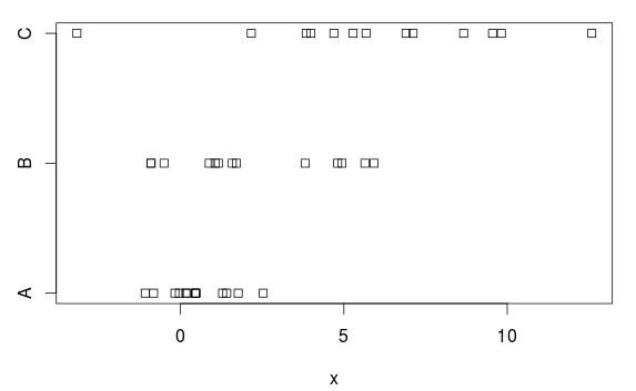
We have three groups, with (clear) differences in both means and variances:

stripchart(x ~ group, data=d)

ANOVA

Not surprisingly, a normal ANOVA handles this quite well:

> mod.aov = aov(x ~ group, data=d)
> summary(mod.aov)
            Df Sum Sq Mean Sq F value  Pr(>F)    
group        2  199.4   99.69   13.01 5.6e-05 ***
Residuals   36  275.9    7.66                    
---
Signif. codes:  0 ‘***’ 0.001 ‘**’ 0.01 ‘*’ 0.05 ‘.’ 0.1 ‘ ’ 1

So, which groups differ? Let’s use Tukey’s HSD method:

> TukeyHSD(mod.aov)
  Tukey multiple comparisons of means
    95% family-wise confidence level

Fit: aov(formula = x ~ group, data = d)

$group
        diff        lwr      upr     p adj
B-A 1.736692 -0.9173128 4.390698 0.2589215
C-A 5.422838  2.7688327 8.076843 0.0000447
C-B 3.686146  1.0321403 6.340151 0.0046867

With a P-value of 0.26, we can’t claim any difference (in means) between group A and B. And even if we didn’t take into account that we did three comparisons, we wouldn’t get a low P-value (P = 0.12):

> summary.lm(mod.aov)
[…]
Coefficients:
            Estimate Std. Error t value  Pr(>|t|)    
(Intercept)   0.5098     0.7678   0.664     0.511    
groupB        1.7367     1.0858   1.599     0.118    
groupC        5.4228     1.0858   4.994 0.0000153 ***
---
Signif. codes:  0 ‘***’ 0.001 ‘**’ 0.01 ‘*’ 0.05 ‘.’ 0.1 ‘ ’ 1

Residual standard error: 2.768 on 36 degrees of freedom

Why is that? Based on the plot, there is a pretty clear difference. The reason is that ANOVA assumes equal variances in each group, and estimates a common standard deviation of 2.77 (shown as ‘Residual standard error’ in the summary.lm table, or you can get it by taking the square root of the residual mean square (7.66) in the ANOVA table).

But group A has a (population) standard deviation of 1, and this overestimate of 2.77 makes it (needlessly) difficult to get statistically significant results, i.e., we have a test with (too) low power.

‘ANOVA’ with unequal variances

So, how to fit a proper model, one that takes into account the differences in variances? It’s easy in R:

> oneway.test(x ~ group, data=d, var.equal=FALSE)
    One-way analysis of means (not assuming equal variances)

data:  x and group
F = 12.7127, num df = 2.000, denom df = 19.055, p-value = 0.0003107

So, if you want to run a simple one-way ‘ANOVA’ in R without assuming equal variances, use this function. It’s basically an extension of the (Welch) t.test() for two samples with unequal variances.

Unfortunately, it doesn’t work with TukeyHSD() (or most other functions you use on aov objects), so even if we’re pretty sure there are group differences, we don’t know where they are.

Modelling the heteroscedasticity

The best solution is to model the variances explicitly. And it’s very easy in R:

> library(nlme)
> mod.gls = gls(x ~ group, data=d,
                weights=varIdent(form= ~ 1 | group))
> anova(mod.gls)
Denom. DF: 36 
            numDF  F-value p-value
(Intercept)     1 16.57316  0.0002
group           2 13.15743  0.0001

Still significant differences, of course. But now the differences between group A and B have also become statically significant (P = 0.025):

> summary(mod.gls)
Generalized least squares fit by REML
  Model: x ~ group
  […]
Variance function:
 Structure: Different standard
            deviations per stratum
 Formula: ~1 | group 
 Parameter estimates:
       A        B        C 
1.000000 2.444532 3.913382 

Coefficients:
               Value Std.Error  t-value p-value
(Intercept) 0.509768 0.2816667 1.809829  0.0787
groupB      1.736692 0.7439273 2.334492  0.0253
groupC      5.422838 1.1376880 4.766542  0.0000
[…]
Residual standard error: 1.015564 
Degrees of freedom: 39 total; 36 residual

So using an appropriate model helps! Also note that we get estimates of the (relative) standard deviations. The estimated standard deviation for group A can be found at the bottom of the, results, 1.02. The estimated standard deviation of group B is 2.44 times this, or 2.48, and the estimated standard deviation of group C is similarly 3.97 (type intervals(mod.gls) to get confidence intervals for the relative standard deviations of groups B and C).

Correcting for multiple testing

However, we really should correct for multiple testing. This is easy using the ‘multcomp’ library. Unfortunately, it does’t have built-in support for ‘gls’ objects, so we’ll have to add some helper functions first:

model.matrix.gls <- function(object, ...)
    model.matrix(terms(object), data = getData(object), ...)
model.frame.gls <- function(object, ...)
  model.frame(formula(object), data = getData(object), ...)
terms.gls <- function(object, ...)
  terms(model.frame(object),...)

Now let’s get to work:

> library(multcomp)
> mod.gls.mc = glht(mod.gls, linfct = mcp(group = "Tukey"))
> summary(mod.gls.mc)
[…]
Linear Hypotheses:
           Estimate Std. Error z value Pr(>|z|)    
B - A == 0   1.7367     0.7439   2.334   0.0480 *  
C - A == 0   5.4228     1.1377   4.767   <0.001 ***
C - B == 0   3.6861     1.2996   2.836   0.0118 *  

Still statistically significant difference between group A and group B! ☺ And we can even get (simultaneous) confidence intervals for the differences between group means:

> confint(mod.gls.mc)
[…]
Linear Hypotheses:
           Estimate lwr     upr    
B - A == 0 1.73669  0.01014 3.46324
C - A == 0 5.42284  2.78242 8.06325
C - B == 0 3.68615  0.66984 6.70245

Using an approximately (here exactly) correct model, we can trust these results!

Note that for this simple example, the data for group C doesn’t really add any information on the differences between group A and B, since we model both separate means and standard deviations for each group. We could have just used pairwise t-tests corrected for multiple comparisons:

> pairwise.t.test(d$x, d$group, pool.sd=FALSE)
    Pairwise comparisons using t tests with non-pooled SD 

data:  d$x and d$group 

  A       B      
B 0.03301 -      
C 0.00098 0.02032

P value adjustment method: holm 

However, for more complicated models, e.g., two-way models, or linear models with many predictors, using GLS (generalised least squares) and explicitly modelling the variance functions is the best solution.

And the variance function need not simply be a different constant in each group; we can impose structure on it. For example, we can model the variance as a power of the mean of each group (and thus only need to estimate one parameter, the exponent), or perhaps as the logarithm of one of the predictors in the model. All this is very easy with GLS (and gls() in R).

Generalised least squares is IMHO a very underused statistical modelling technique. Instead of worrying about deviations from the model assumptions, model those deviations!

Answer 3

1. There may indeed be some transformation of your data that produces an acceptably normal distribution. Of course, now your inference is about about the transformed data, not the not-transformed data.

2. Assuming you are talking about a oneway ANOVA, the Kruskal-Wallis test is an appropriate nonparametric analog to the oneway ANOVA. Dunn's test (not the garden-variety rank sum test) is perhaps the most common nonparametric test appropriate for post hoc pair-wise multiple comparisons, although there are other tests such as the Conover-Iman test (strictly more powerful than Dunn's test after rejection of the kruskal-Wallis), and the Dwass-Steele-Crichtlow-Fligner test.

3. Multiple comparisons procedures (whether family-wise error rate variety or false discovery rate variety) don't really have anything directly to do with your specific test assumptions (e.g., normality of data), rather they have to do with the meaning of $\alpha$ (willingness to make a false rejection of a null hypothesis) given that you are performing multiple tests.

The ANOVA is based on a ratio of within group and between group variances. I am not entirely sure what you mean by heteroscedasticity in this context, but if you mean unequal variances between groups, that would seem to me to fundamentally break the logic of the test's null hypothesis.

A simple Google Scholar query for "Dunn's test" along with a general term from your discipline should return plenty of published examples.

References

Conover, W. J. and Iman, R. L. (1979). On multiple-comparisons procedures. Technical Report LA-7677-MS, Los Alamos Scientific Laboratory.

Crichtlow, D. E. and Fligner, M. A. (1991). On distribution-free multiple comparisons in the one-way analysis of variance. Communications in Statistics—Theory and Methods, 20(1):127.

Dunn, O. J. (1964). Multiple comparisons using rank sums. Technometrics, 6(3):241–252.

Answer 4

It sounds to me as though you are doing the footwork and are trying your best but are worried your efforts will not be good enough to get your paper past the reviewers. Very much a real-world problem. I think all researchers struggle with analyses that appear to be borderline or even frankly breaching assumptions from time to time. After all there are millions of articles evaluating e.g. treatment effects in 3 small groups of mice with something like 6 - 7 mice in each group. How to know if Anova assumptions are satisfied in such a paper!

I have reviewed a large number of papers especially in the field of cardiovascular pathophysiology and actually never do feel 100% sure whether I can trust the data or not in an article that I read. But for me as a reviewer, I actually tend to think that issues can arise at so many levels in science that there is probably little point in digging too deep into the statistics -- after all, the whole dataset could be fabricated and I would never in a million years be able to tell. Accordingly, there will always be an element of trust in this field of work, which researchers must never abuse.

The most real-world suggestion I would give is that you need to think everything through very carefully before you submit and make sure you will be able to answer truthfully any questions asked by the reviewers. As long as you have done your best, your intentions are honest and you sleep well at night I think you should be ok.