4
$\begingroup$

In ordinary least squares regression (OLS), if the plot of the residuals against the fitted values form a horizontal line around 0, then we can say that the dependent variable is linearly related to the independent variable.

I had thought that this is true because $E(y_i - \hat{y}_I)=0$ when the dependent variable is linearly related to the independent variable, see here.

However, suppose:

$y_i = \alpha + \sin(x_i) + \epsilon_i$.

Then $E(y_i - \hat{y}_i)$ is still 0, see here but then the plot of its residuals against its fitted value is no longer a horizontal line around 0, as this R code shows:

n <- 10^3
df <- data.frame(x=runif(n, 1, 10))
df$mean.y.given.x <- sin(df$x)
df$y <- df$mean.y.given.x + rnorm(n)
model <- lm(y ~ x, data=df)
plot(predict(model, newdata=df), residuals(model))
abline(a=0,b=0,col='blue')
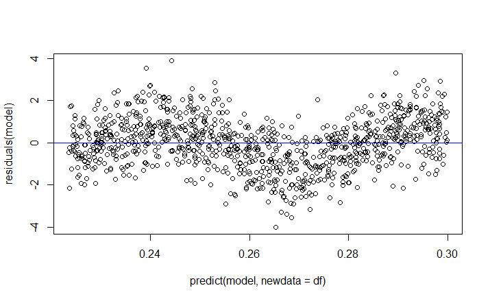
enter image description here

So my question is, which assumption(s) of OLS that causes the plot of the residuals and the fitted value to be a horizontal line around 0 and why/how is it true?

$\endgroup$
4
  • 2
    $\begingroup$ You've regressed $y$ on $x$, not on $\sin x$. $\endgroup$
    – Scortchi
    Commented May 31, 2014 at 11:09
  • $\begingroup$ @Scortchi Are you referring to the R code or the expression $E(y_i-\hat{y_i})=0$? Could you please show me how to regress it on $\sin x$? $\endgroup$
    – mauna
    Commented May 31, 2014 at 11:26
  • 2
    $\begingroup$ In the statement model <- lm(y ~ x, data=df) substitute sin(x) for x $\endgroup$
    – Peter Flom
    Commented May 31, 2014 at 12:07
  • 3
    $\begingroup$ The R code - though I'd overlooked that the model equation you gave doesn't in fact include an coefficient for $\sin x$, as explained by @Glen_b. In any case, a correctly specified model is a necessary assumption for the residuals to behave as expected with OLS, & the point of plotting residuals vs fits is to look for signs of mis-specification. $\endgroup$
    – Scortchi
    Commented Jun 1, 2014 at 10:50

1 Answer 1

7
$\begingroup$

Scortchi and Peter Flom have both correctly pointed out that you didn't fit the model you specified.

However, there's no coefficient on $\sin(x)$ in the model, so if you actually want to fit $y_i = \alpha + \sin(x_i) + \epsilon_i$ you should not regress on $\sin(x)$. In that model it's an offset, not a regressor.

The correct way to specify the model

$$y_i = \alpha + \sin(x_i) + \epsilon_i$$

in R is:

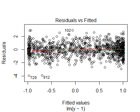
model <- lm(y ~ 1, offset=sin(x), data=df)

which produces the residual vs fitted plot:
enter image description here

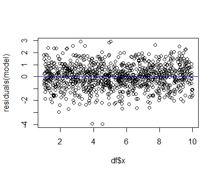
or as a residuals vs x plot:
enter image description here

Alternatively, one could fit

model2 <- lm( y-sin(x) ~ 1, data=df)

which gives the same estimate for $\alpha$. The residual vs fitted plot is of no use in this case (because of the difference in the way the offset was brought into the model by modifying $y$), but the residuals vs x plot is identical to the second plot above.


Gung is right to suggest in comments that it often makes sense to fit the offset as a regressor anyway (for example, to check that the offset-coefficient of 1 is reasonable); this is the model that Scortchi and Peter Flom were discussing in comments.

Here's how you do that:

model3 <- lm( y ~ sin(x), data=df)

If we look at the summary (summary(model3)) we get:

Coefficients:
            Estimate Std. Error t value Pr(>|t|)    
(Intercept) 0.000717   0.032050   0.022    0.982    
sin(x)      1.069593   0.044947  23.797   <2e-16 ***
---
Signif. codes:  0 ‘***’ 0.001 ‘**’ 0.01 ‘*’ 0.05 ‘.’ 0.1 ‘ ’ 1

Residual standard error: 0.9921 on 998 degrees of freedom
Multiple R-squared:  0.362, Adjusted R-squared:  0.3614 
F-statistic: 566.3 on 1 and 998 DF,  p-value: < 2.2e-16

which has coefficients close to what we'd expect.

Finally, you might do this:

model4 <- lm( y ~ sin(x),offset=sin(x), data=df)

but its effect is only to reduce the fitted coefficient of $\sin(x)$ by 1, so we can extract the same information from model3's output.

$\endgroup$
3
  • $\begingroup$ thank you for your answer. Actually, I just completed my degree's introductory statistics course. Could you please recommend some textbooks that covers the concepts in your answer? E.g. I have never come across the term 'offset' before. $\endgroup$
    – mauna
    Commented Jun 1, 2014 at 20:54
  • 1
    $\begingroup$ The use of the term 'offset' is most commonly encountered when discussing generalized linear models (GLMs). The concept exists in ordinary regression, but since it's so easy to just adjust $y$ for fixed-coefficient terms instead (as I did with model2 above), people often don't run into it until they deal with GLMs (where you generally can't just adjust the data in that fashion) and almost any decent introduction to GLMs discuss the idea. Fox & Weisberg's An R Companion to Applied Regression does cover the use of an offset in regression in R. $\endgroup$
    – Glen_b
    Commented Jun 2, 2014 at 0:13
  • 2
    $\begingroup$ However, when dealing with a fixed-coefficient term, if the idea of moving from $y=\alpha+\sin(x)+\epsilon$ to $y^* =\alpha+\epsilon$ where $y^*=y-\sin(x)$, and then using $\hat y = \hat y^*+\sin(x)$ makes sense to you, you don't really need any special concepts to deal with offsets. $\endgroup$
    – Glen_b
    Commented Jun 2, 2014 at 0:17

Your Answer

By clicking “Post Your Answer”, you agree to our terms of service and acknowledge you have read our privacy policy.

Not the answer you're looking for? Browse other questions tagged or ask your own question.