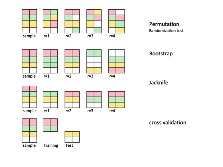
We can find different Resampling methods, or loosely called "simulation" methods, that depend upon resampling or shuffling of the samples. There might be differences in opinions with respect to proper terminology, but the following discussion tries to generalize and simplify what is available in the appropriate literature:
Resampling methods are used in (1) estimating precision / accuracy of sample statistics through using subset of data (e.g. Jackknifing) or drawing randomly with replacement from a set of data points (e.g. bootstrapping) (2) Exchanging labels on data points when performing significance tests (permutation tests, also called exact tests, randomization tests, or re-randomization tests) (3) Validating models by using random subsets (bootstrapping, cross validation) (see wikipedia: resampling methods)
BOOTSTRAPING
"Bootstrapping is a statistical method for estimating the sampling distribution of an estimator by sampling with replacement from the original sample". The method assigns measures of accuracy (defined in terms of bias, variance, confidence intervals, prediction error or some other such measure) to sample estimates.
The basic idea of bootstrapping is that inference about a population from sample data (sample → population) can be modeled by resampling the sample data and performing inference on (resample → sample). As the population is unknown, the true error in a sample statistic against its population value is unknowable. In bootstrap-resamples, the 'population' is in fact the sample, and this is known; hence the quality of inference from resample data → 'true' sample is measurable." see wikipedia
Yvar <- c(8,9,10,13,12, 14,18,12,8,9, 1,3,2,3,4)
#To generate a single bootstrap sample
sample(Yvar, replace = TRUE)
#generate 1000 bootstrap samples
boot <-list()
for (i in 1:1000)
boot[[i]] <- sample(Yvar,replace=TRUE)
In univariate problems, it is usually acceptable to resample the individual observations with replacement ("case resampling"). Here we resample the data with replacement, and the size of the resample must be equal to the size of the original data set.
In regression problems, case resampling refers to the simple scheme of resampling individual cases - often rows of a data set in regression problems, the explanatory variables are often fixed, or at least observed with more control than the response variable. Also, the range of the explanatory variables defines the information available from them. Therefore, to resample cases means that each bootstrap sample will lose some information (see Wikipedia). So it will be logical to sample rows of the data rather just Yvar.
Yvar <- c(8,9,10,13,12, 14,18,12,8,9,   1,3,2,3,4)
Xvar <- c(rep("A", 5),  rep("B", 5),    rep("C", 5))
mydf <- data.frame (Yvar, Xvar)
boot.samples <- list()
for(i in 1:10) {
b.samples.cases <- sample(length(Xvar), length(Xvar), replace=TRUE)
b.mydf <- mydf[b.samples.cases,]
boot.samples[[i]] <- b.mydf
}
str(boot.samples)
boot.samples[1]
You can see some cases are repeated as we are sampling with replacement.
"Parametric bootstrap - a parametric model is fitted to the data, often by maximum likelihood, and samples of random numbers are drawn from this fitted model. Usually the sample drawn has the same sample size as the original data. Then the quantity, or estimate, of interest is calculated from these data. This sampling process is repeated many times as for other bootstrap methods. The use of a parametric model at the sampling stage of the bootstrap methodology leads to procedures which are different from those obtained by applying basic statistical theory to inference for the same model."(see Wikipedia). The following is parametric bootstrap with normal distribution assumption with mean and standard deviation parameters.
Yvar <- c(8,9,10,13,12, 14,18,12,8,9,   1,3,2,3,4)

# parameters for Yvar
mean.y <- mean(Yvar)
sd.y <- sd(Yvar)

#To generate a single bootstrap sample with assumed normal distribution (mean, sd)
rnorm(length(Yvar), mean.y, sd.y)

 #generate 1000 bootstrap samples
boot <-list()
for (i in 1:1000)
   boot[[i]] <- rnorm(length(Yvar), mean.y, sd.y)
There are other variants of bootstrap, please consult the wikipedia page or any good statical book on resampling.
JACKNIFE
"The jackknife estimator of a parameter is found by systematically leaving out each observation from a dataset and calculating the estimate and then finding the average of these calculations. Given a sample of size N, the jackknife estimate is found by aggregating the estimates of each N − 1 estimate in the sample." see: wikipedia The following shows how to jackknife the Yvar.
jackdf <- list()
jack <- numeric(length(Yvar)-1)

for (i in 1:length (Yvar)){

for (j in 1:length(Yvar)){
     if(j < i){
            jack[j] <- Yvar[j]
}  else if(j > i) {
             jack[j-1] <- Yvar[j]
}
}
jackdf[[i]] <- jack
}
jackdf
"the regular bootstrap and the jackknife, estimate the variability of a statistic from the variability of that statistic between subsamples, rather than from parametric assumptions. For the more general jackknife, the delete-m observations jackknife, the bootstrap can be seen as a random approximation of it. Both yield similar numerical results, which is why each can be seen as approximation to the other." See this question on Bootstrap vs Jacknife.
RANDOMIZATION TESTS
"In parametric tests we randomly sample from one or more populations. We make certain assumptions about those populations, most commonly that they are normally distributed with equal variances. We establish a null hypothesis that is framed in terms of parameters, often of the form m1 -m2 = 0 . We use our sample statistics as estimates of the corresponding population parameters, and calculate a test statistic (such as a t test). For example: in Student's t - test for differences in means when variances are unknown, but are considered to be equal. The hypothesis of interest is that H0: m1 = m2. One of alternative hypothesis would be stated as : HA: m1 < m2.
Given two samples drawn from populations 1 and 2, assuming that these are normally distributed populations with equal variances, and that the samples were drawn independently and at random from each population, then a statistic whose distribution is known can be elaborated to test H0.
One way to avoid these distributional assumptions has been the approach now called non - parametric, rank - order, rank - like, and distribution - free statistics. These distribution - free statistics are usually criticized for being less "efficient" than the analogous test based on assuming the populations to be normally distributed.
Another alternative approach is randomization approach - "process of randomly assigning ranks to observations independent of one's knowledge of which sample an observation is a member. A randomization test makes use of such a procedure, but does so by operating on the observations rather than the joint ranking of the observations. For this reason, the distribution of an analogous statistic (the sum of the observations in one sample) cannot be easily tabulated, although it is theoretically possible to enumerate such a distribution" (see)
Randomization tests differ from parametric tests in almost every respect. (1) There is no requirement that we have random samples from one or more populations—in fact we usually have not sampled randomly. (2) We rarely think in terms of the populations from which the data came, and there is no need to assume anything about normality or homoscedasticity (3) Our null hypothesis has nothing to do with parameters, but is phrased rather vaguely, as, for example, the hypothesis that the treatment has no effect on the how participants perform.(4) Because we are not concerned with populations, we are not concerned with estimating (or even testing) characteristics of those populations (5) We do calculate some sort of test statistic, however we do not compare that statistic to tabled distributions. Instead, we compare it to the results we obtain when we repeatedly randomize the data across the groups, and calculate the corresponding statistic for each randomization. (6) Even more than parametric tests, randomization tests emphasize the importance of random assignment of participants to treatments." see.
The type of randomization test that is very popular is permutation test. If our sample size is 12 and 5, the total permutation possible is C(12,5) = 792. If our sample sizes been 10 and 15 then over 3.2 million arrangements would have been possible. This is computing challenge: What then? Sample. When the universe of possible arrangements is too large to enumerate why not sample arrangements from this universe independently and at random? The distribution of the test statistic over this series of samples can then be tabulated, its' mean and variance computed, and the error rate associated with an hypothesis test estimated.
PERMUTATION TEST
According to wikipedia "A permutation test (also called a randomization test, re-randomization test, or an exact test) is a type of statistical significance test in which the distribution of the test statistic under the null hypothesis is obtained by calculating all possible values of the test statistic under rearrangements of the labels on the observed data points. Permutation tests exist for any test statistic, regardless of whether or not its distribution is known. Thus one is always free to choose the statistic which best discriminates between hypothesis and alternative and which minimizes losses."
The difference between permutation and bootstrap is that bootstraps sample with replacement, and permutations sample without replacement. In either case, the time order of the observations is lost and hence volatility clustering is lost — thus assuring that the samples are under the null hypothesis of no volatility clustering.
The permutations always have all of the same observations, so they are more like the original data than bootstrap samples. The expectation is that the permutation test should be more sensitive than a bootstrap test. The permutations destroy volatility clustering but do not add any other variability.
See the question on permutation vs bootstrapping - "The permutation test is best for testing hypotheses and bootstrapping is best for estimating confidence intervals".
So to perform permutation in this case we can just change replace = FALSE in the above bootstrap example.
Yvar <- c(8,9,10,13,12, 14,18,12,8,9,   1,3,2,3,4)
     #generate 1000 bootstrap samples
       permutes <-list()
    for (i in 1:1000)
       permutes[[i]] <- sample(Yvar,replace=FALSE)
In case of more than one variable, just picking of the rows and reshuffling the order will not make any difference as the data will remain same. So we reshuffle the y variable. Something what you have done, but I do not think we need double reshuffling of both x and y variables (as you have done).
Yvar <- c(8,9,10,13,12, 14,18,12,8,9,   1,3,2,3,4)
Xvar <- c(rep("A", 5),  rep("B", 5),    rep("C", 5))
mydf <- data.frame (Yvar, Xvar)

 permt.samples <- list()
    for(i in 1:10) {
       t.yvar <- Yvar[ sample(length(Yvar), length(Yvar), replace=FALSE) ]
       b.df <- data.frame (Xvar, t.yvar)
       permt.samples[[i]] <- b.df
    }
    str(permt.samples)
    permt.samples[1]
MONTE CARLO METHODS
"Monte Carlo methods (or Monte Carlo experiments) are a broad class of computational algorithms that rely on repeated random sampling to obtain numerical results; typically one runs simulations many times over in order to obtain the distribution of an unknown probabilistic entity. The name comes from the resemblance of the technique to the act of playing and recording results in a real gambling casino. " see Wikipedia
"In applied statistics, Monte Carlo methods are generally used for two purposes:
(1) To compare competing statistics for small samples under realistic data conditions. Although Type I error and power properties of statistics can be calculated for data drawn from classical theoretical distributions (e.g., normal curve, Cauchy distribution) for asymptotic conditions (i. e, infinite sample size and infinitesimally small treatment effect), real data often do not have such distributions.
(2) To provide implementations of hypothesis tests that are more efficient than exact tests such as permutation tests (which are often impossible to compute) while being more accurate than critical values for asymptotic distributions.
Monte Carlo methods are also a compromise between approximate randomization and permutation tests. An approximate randomization test is based on a specified subset of all permutations (which entails potentially enormous housekeeping of which permutations have been considered). The Monte Carlo approach is based on a specified number of randomly drawn permutations (exchanging a minor loss in precision if a permutation is drawn twice – or more frequently—for the efficiency of not having to track which permutations have already been selected)."
Both MC and Permutation test are sometime collectively called randomization tests. The difference is in MC we sample the permutation samples, rather using all possible combinations [see] 21.
CROSS VALIDATION
The idea beyond cross validation is that models should be tested with data that were not used to fit the model. Cross validation is perhaps most often used in the context of prediction.
"Cross-validation is a statistical method for validating a predictive model. Subsets of the data are held out for use as validating sets; a model is fit to the remaining data (a training set) and used to predict for the validation set. Averaging the quality of the predictions across the validation sets yields an overall measure of prediction accuracy.
One form of cross-validation leaves out a single observation at a time; this is similar to the jackknife. Another, K-fold cross-validation, splits the data into K subsets; each is held out in turn as the validation set." see Wikipedia . Cross validation is usually done with quantitative data. You can convert your qualitative (factor data) to quantitative someway to fit a linear model and test this model. The following is simple hold-out strategy where 50% of data is used for model prediction while rest is used for testing. Lets assume Xvar is also quantitative variable.
    Yvar <- c(8,9,10,13,12, 14,18,12,8,9,   1,3,2,3,4)
    Xvar <- c(rep(1, 5),  rep(2, 5),    rep(3, 5))
    mydf <- data.frame (Yvar, Xvar)
    training.id <- sample(1:nrow(mydf), round(nrow(mydf)/2,0), replace = FALSE)
    test.id <- setdiff(1:nrow(mydf), training.id)
   # training dataset
    mydf.train <- mydf[training.id]

    #testing dataset
    mydf.test <- mydf[test.id]
Unlike bootstrap and permutation tests the cross-validation dataset for training and testing is different. The following figure shows a summary of resampling in different methods.

Hope this helps a bit.


